OPICO 5: Tuning Recursive SQL for Item/Category Optimization
Part 5 in a series on: Optimization Problems with Items and Categories in Oracle
In the fourth article, we explained how to use recursive SQL to implement the algorithms described generically in the third, including the Value Filtering techniques that will prove essential here.
In the current article, we introduce two larger test datasets and use them to analyse the performance of the initial recursive query, then go on to look at variations on the query that improve performance.
The performance results cited are from instance 3 of running the driver script, Run-All.ps1: Run-All_03.log (summary) and results_03 folder (detail) in the GitHub project

[Image by Fran Soto from Pixabay]
Contents
↓ 1 Test Datasets - Fantasy Football
↓ 2 Value Filtering Parameters
↓ 3 Pure Recursive SQL
↓ 4 Recursive SQL with PL/SQL
↓ 5 Conclusion
1 Test Datasets - Fantasy Football
↑ Contents
↓ Solutions by Position Query
↓ Test Dataset 1: Brazilian League
↓ Test Dataset 2: English Premier League
In the previous article a very simple demo problem involving 6 items and 2 categories was used for illustrative purposes. We need larger problems to analyse performance, and in this section two problems are described, each of them based on the concept of fantasy football: Here the items are footballers, whose playing positions form the categories, and the players have prices whose total for a team has a maximum limit, and values based on their anticipated ability to generate points for the team.
Before describing the test datasets, we show a query that allows us to list solutions arranged by position with minimum and maximum limits and the actual number in the position, with player ids as comma-separated lists inline. It is convenient for quickly verifying that all the category limits have been adhered to.
Solutions by Position Query
↑ 1 Test Datasets - Fantasy Football
The query applies to solutions accessed via a view, PATHS_RANKED_V, that stores the solutions as strings containing a list of player ids of fixed length in a PATH column, and relies on a splitting function, Item_Cat_Seqs.Split_Values. It uses the Oracle aggregate function, ListAgg.
SELECT prv.tot_value,
       prv.tot_price,
       prv.rnk,
       cat.id                 category_id,
       To_Char(cat.min_items) min_items,
       ' ' || CASE WHEN COUNT(itm.id) = cat.min_items THEN '<-' ELSE '  ' END || COUNT(itm.id) ||
          CASE WHEN COUNT(itm.id) = cat.max_items THEN '->' ELSE '  ' END n_items,
       To_Char(cat.max_items) max_items,
       ListAgg(itm.id, ', ')  item_list
  FROM categories cat
 CROSS JOIN paths_ranked_v prv
 CROSS APPLY TABLE(Item_Cat_Seqs.Split_Values(prv.path, :ITEM_WIDTH)) psv
  LEFT JOIN items itm ON itm.id = psv.COLUMN_VALUE
   AND itm.category_id = cat.id
 WHERE prv.rnk <= :TOP_N
 GROUP BY prv.tot_value,
          prv.tot_price,
          prv.rnk,
          cat.id,
          cat.min_items,
          cat.max_items
 ORDER BY 3, 4
Test Dataset 1: Brazilian League
↑ 1 Test Datasets - Fantasy Football
↓ Test Dataset
↓ Path Level Solutions, with Statistics
↓ Item Level Solutions
↓ Solutions by Position
The first dataset was supplied by a post on Processing Cost - How to catch a soccer team with the highest combined score? and appears to be based on a Brazilian league.
Test Dataset
↑ Test Dataset 1: Brazilian League
The dataset has 114 players, in seven positions (one being coach), with twelve players forming a team. The problem is to find the team with maximum total player points within a given maximum price (of 19000), and matching the positional constraints:
Positions

Position     Min Players    Max Players
--------- -------------- --------------
AL                    12             12
CB                     2              3
CO                     1              1
FW                     1              3
GK                     1              1
MF                     3              5
WB                     0              2

7 rows selected.

Players

Position  Id  Player                Player Price Player Value
--------- --- --------------------- ------------ ------------
CB        098 Digão                          931          927
          099 Samir                          267          680
          100 Dedé                          2254          640
          101 Lúcio                         2171          602
          102 Bressan                       1085          590
          103 Manoel                        1699          588
          104 Cléber                        1461          578
          105 Bruno Rodrigo                 1547          528
          106 Edu Dracena                   1682          497
          107 William Alves                  556          443
          108 Gum                           1218          422
          109 Wallace                        429          420
          110 João Filipe                    547          410
          111 Werley                        1590          403
          112 Gil                           1323          398
          113 Gabriel Paulista              1177          394
          114 Ernando                       1024          374
CO        078 Jaime De AlMFda               1156          803
          079 Marcelo Oliveira              1611          543
          080 Abel Braga                    1751          536
          081 Dunga                         1422          463
          082 Caio Júnior                   1140          445
          083 Vanderlei Luxemburgo          1577          442
          084 Ney Franco                    1515          439
          085 Levi Gomes                     708          420
          086 Ricardo Drubscky               796          392
          087 Marquinhos Santos             1059          389
          088 Paulo Autuori                 1313          361
          089 Edson Pimenta                  367          326
          090 Oswaldo De Oliveira           1077          323
          091 Tite                          1368          317
          092 Claudinei Oliveira            1192          317
          093 Cristóvão Borges               827          292
          094 Vadão                          704          286
          095 Enderson Moreira               680          253
          096 Cuca                          1262          232
          097 Zé Sérgio                      685           75
FW        001 Éderson                       1712         1012
          002 Maxi Biancucchi               1962         1005
          003 Rafael Sobis                  2303          955
          004 Fernandão                     1328          822
          005 Luis Fabiano                  2154          758
          006 Rafael Marques                1974          668
          007 Dagoberto                     2211          594
          008 Rogério                       1062          570
          009 Hernane                       1387          498
          010 Lins                          1840          490
          011 Neilton                        638          488
          012 Samuel                        1001          487
          013 Chiquinho                      997          464
          014 Luan                          1318          455
          015 William                       1393          444
          016 Vitinho                       1020          404
          017 Deivid                        1590          376
          018 Barcos                        1896          367
          019 Jô                            1393          340
          020 Osvaldo                       1364          312
GK        021 Fábio                         2090          794
          022 Wilson                        1239          794
          023 Vanderlei                     1858          776
          024 Victor                        1163          467
          025 Marcelo Lomba                 1364          450
          026 Renan                          677          437
          027 Felipe                        1526          414
          028 Dida                          1132          375
          029 Cássio                        1251          374
          030 Michel Alves                   899          348
          031 Bruno                         1066          320
          032 Muriel                         981          310
          033 Rafael                        1782          300
          034 Weverton                       616          248
          035 Ricardo Berna                  460          242
          036 Gledson                        452          210
          037 Rogério Ceni                  1420          117
MF        058 Fred                          3028          892
          059 Zé Roberto                    2593          878
          060 Otavinho                       762          807
          061 Carlos Alberto                1501          675
          062 Nilton                        2239          646
          063 Júnior Urso                   1438          622
          064 João Vitor                    1327          604
          065 Guilherme                      883          587
          066 Ralf                          1965          570
          067 Escudero                      1638          568
          068 Correa                         844          560
          069 Souza                         1262          517
          070 Alex                          1698          508
          071 Souza                         1380          498
          072 Cicinho                       1142          472
          073 Fellype Gabriel                860          447
          074 João Paulo                    1056          438
          075 Sandro Silva                  1076          428
          076 Cícero                        1415          418
          077 Wagner                         855          413
WB        038 Ivan                           755         1320
          039 Elsinho                       1468          850
          040 Egídio                        1482          752
          041 Carlinhos                     1240          693
          042 Auremir                        773          548
          043 Mayke                          374          525
          044 Luis Ricardo                   858          467
          045 Richarlyson                   1020          467
          046 Fabrício                       876          457
          047 Juan                           789          457
          048 Paulo Miranda                 1053          454
          049 João Paulo                     715          453
          050 Rodrigo Caio                  1192          452
          051 Victor Ferraz                 1304          420
          052 Jussandro                      694          410
          053 Rafael Galhardo               1288          404
          054 William Matheus                587          402
          055 Maranhão                       653          402
          056 Gabriel                       1181          338
          057 Vítor                          877          336

114 rows selected.
AL is used as a code for team size, and a maximum price of 19000 was chose arbitrarily (but having an influence on results). The points and prices were multiplied by a factor of 100 to allow working in integers.
Path Level Solutions, with Statistics
↑ Test Dataset 1: Brazilian League
Running the pure SQL recursive query of the last article by means of a view, RSF_SQL_V, on the Brazil dataset with KEEP_NUM = 10 and MIN_VALUE = 0, we get a solution set for the top 10 paths that is suboptimal (let’s call it B-B), summarised below:
| KEEP_NUM | MIN_VALUE | Solution Set | Value 1 | Value 10 | Seconds |
|---|---|---|---|---|---|
| 10 | 0 | B-B (suboptimal) | 10923 | 10748 | 0.9 |
Path                                 Total Value Total Price  Rank
------------------------------------ ----------- ----------- -----
078022098099058059060001002003038039       10923       18176     1
078023098099058059060001002003038039       10905       18795     2
078022098099058059060001002003038040       10825       18190     3
078023098099058059060001002003038040       10807       18809     4
078022098099058059060001002004038039       10790       17201     5
078021098099058059060001002004038039       10790       18052     6
078023098099058059060001002004038039       10772       17820     7
078022098099058059060001002003038041       10766       17948     8
078021098099058059060001002003038041       10766       18799     9
078022098099058059060061001002003038       10748       18209    10

10 rows selected.

Elapsed: 00:00:00.87
The query executes in less than a second, finding the best solution with value of 10923, but the remaining solutions miss some better solutions, as shown when we run for a value of KEEP_NUM = 0, meaning ‘do not approximate’, and using a MIN_VALUE of 10748, since we know from the above run that the 10’th best solution has a value at least that high:
| KEEP_NUM | MIN_VALUE | Solution Set | Value 1 | Value 10 | Seconds |
|---|---|---|---|---|---|
| 100 | 10748 | B-A (optimal) | 10923 | 10766 | 1.0 |
Path                                 Total Value Total Price  Rank
------------------------------------ ----------- ----------- -----
078022098099058059060001002003038039       10923       18176     1
078023098099058059060001002003038039       10905       18795     2
078022098102058059060001002003038039       10833       18994     3
078022098099058059060001002003038040       10825       18190     4
078023098099058059060001002003038040       10807       18809     5
078022098099058059061001002003038039       10791       18915     6
078022098099058059060001002004038039       10790       17201     7
078021098099058059060001002004038039       10790       18052     8
078023098099058059060001002004038039       10772       17820     9
078022098099058059060001002003038041       10766       17948    10

10 rows selected.

Elapsed: 00:00:01.03
This takes only slightly longer at 1.0 seconds because the lower bound on the 10’th best solution value allows the search algorithm to truncate some of the paths, and finds the best solution set (let’s call it B-A) since it is not approximating at all.
Item Level Solutions
↑ Test Dataset 1: Brazilian League
Here is the best solution set found, with paths split into items and joined to the players:
Total Value Total Price Rank Position Item Player Value Price
----------- ----------- ----- -------- ---- ------------------------------ ---------- ----------
10923 18176 1 CO 078 Jaime De AlMFda 803 1156
GK 022 Wilson 794 1239
CB 098 Digão 927 931
099 Samir 680 267
MF 058 Fred 892 3028
059 Zé Roberto 878 2593
060 Otavinho 807 762
FW 001 Éderson 1012 1712
002 Maxi Biancucchi 1005 1962
003 Rafael Sobis 955 2303
WB 038 Ivan 1320 755
039 Elsinho 850 1468
10905 18795 2 CO 078 Jaime De AlMFda 803 1156
GK 023 Vanderlei 776 1858
CB 098 Digão 927 931
099 Samir 680 267
MF 058 Fred 892 3028
059 Zé Roberto 878 2593
060 Otavinho 807 762
FW 001 Éderson 1012 1712
002 Maxi Biancucchi 1005 1962
003 Rafael Sobis 955 2303
WB 038 Ivan 1320 755
039 Elsinho 850 1468
10833 18994 3 CO 078 Jaime De AlMFda 803 1156
GK 022 Wilson 794 1239
CB 098 Digão 927 931
102 Bressan 590 1085
MF 058 Fred 892 3028
059 Zé Roberto 878 2593
060 Otavinho 807 762
FW 001 Éderson 1012 1712
002 Maxi Biancucchi 1005 1962
003 Rafael Sobis 955 2303
WB 038 Ivan 1320 755
039 Elsinho 850 1468
10825 18190 4 CO 078 Jaime De AlMFda 803 1156
GK 022 Wilson 794 1239
CB 098 Digão 927 931
099 Samir 680 267
MF 058 Fred 892 3028
059 Zé Roberto 878 2593
060 Otavinho 807 762
FW 001 Éderson 1012 1712
002 Maxi Biancucchi 1005 1962
003 Rafael Sobis 955 2303
WB 038 Ivan 1320 755
040 Egídio 752 1482
10807 18809 5 CO 078 Jaime De AlMFda 803 1156
GK 023 Vanderlei 776 1858
CB 098 Digão 927 931
099 Samir 680 267
MF 058 Fred 892 3028
059 Zé Roberto 878 2593
060 Otavinho 807 762
FW 001 Éderson 1012 1712
002 Maxi Biancucchi 1005 1962
003 Rafael Sobis 955 2303
WB 038 Ivan 1320 755
040 Egídio 752 1482
10791 18915 6 CO 078 Jaime De AlMFda 803 1156
GK 022 Wilson 794 1239
CB 098 Digão 927 931
099 Samir 680 267
MF 058 Fred 892 3028
059 Zé Roberto 878 2593
061 Carlos Alberto 675 1501
FW 001 Éderson 1012 1712
002 Maxi Biancucchi 1005 1962
003 Rafael Sobis 955 2303
WB 038 Ivan 1320 755
039 Elsinho 850 1468
10790 17201 7 CO 078 Jaime De AlMFda 803 1156
GK 022 Wilson 794 1239
CB 098 Digão 927 931
099 Samir 680 267
MF 058 Fred 892 3028
059 Zé Roberto 878 2593
060 Otavinho 807 762
FW 001 Éderson 1012 1712
002 Maxi Biancucchi 1005 1962
004 Fernandão 822 1328
WB 038 Ivan 1320 755
039 Elsinho 850 1468
18052 8 CO 078 Jaime De AlMFda 803 1156
GK 021 Fábio 794 2090
CB 098 Digão 927 931
099 Samir 680 267
MF 058 Fred 892 3028
059 Zé Roberto 878 2593
060 Otavinho 807 762
FW 001 Éderson 1012 1712
002 Maxi Biancucchi 1005 1962
004 Fernandão 822 1328
WB 038 Ivan 1320 755
039 Elsinho 850 1468
10772 17820 9 CO 078 Jaime De AlMFda 803 1156
GK 023 Vanderlei 776 1858
CB 098 Digão 927 931
099 Samir 680 267
MF 058 Fred 892 3028
059 Zé Roberto 878 2593
060 Otavinho 807 762
FW 001 Éderson 1012 1712
002 Maxi Biancucchi 1005 1962
004 Fernandão 822 1328
WB 038 Ivan 1320 755
039 Elsinho 850 1468
10766 17948 10 CO 078 Jaime De AlMFda 803 1156
GK 022 Wilson 794 1239
CB 098 Digão 927 931
099 Samir 680 267
MF 058 Fred 892 3028
059 Zé Roberto 878 2593
060 Otavinho 807 762
FW 001 Éderson 1012 1712
002 Maxi Biancucchi 1005 1962
003 Rafael Sobis 955 2303
WB 038 Ivan 1320 755
041 Carlinhos 693 1240
120 rows selected.
Solutions by Position
↑ Test Dataset 1: Brazilian League
Here is the best solution set found, arranged by position, with player ids listed inline:
Total Value Total Price  Rank Position Min Actual  Max Player List
----------- ----------- ----- -------- --- ------- --- -------------------------
      10923       18176     1 CB       2    <-2    3   098, 099
                              CO       1    <-1->  1   078
                              FW       1      3->  3   001, 002, 003
                              GK       1    <-1->  1   022
                              MF       3    <-3    5   058, 059, 060
                              WB       0      2->  2   038, 039
      10905       18795     2 CB       2    <-2    3   098, 099
                              CO       1    <-1->  1   078
                              FW       1      3->  3   001, 002, 003
                              GK       1    <-1->  1   023
                              MF       3    <-3    5   058, 059, 060
                              WB       0      2->  2   038, 039
      10833       18994     3 CB       2    <-2    3   098, 102
                              CO       1    <-1->  1   078
                              FW       1      3->  3   001, 002, 003
                              GK       1    <-1->  1   022
                              MF       3    <-3    5   058, 059, 060
                              WB       0      2->  2   038, 039
      10825       18190     4 CB       2    <-2    3   098, 099
                              CO       1    <-1->  1   078
                              FW       1      3->  3   001, 002, 003
                              GK       1    <-1->  1   022
                              MF       3    <-3    5   058, 059, 060
                              WB       0      2->  2   038, 040
      10807       18809     5 CB       2    <-2    3   098, 099
                              CO       1    <-1->  1   078
                              FW       1      3->  3   001, 002, 003
                              GK       1    <-1->  1   023
                              MF       3    <-3    5   058, 059, 060
                              WB       0      2->  2   038, 040
      10791       18915     6 CB       2    <-2    3   098, 099
                              CO       1    <-1->  1   078
                              FW       1      3->  3   001, 002, 003
                              GK       1    <-1->  1   022
                              MF       3    <-3    5   058, 059, 061
                              WB       0      2->  2   038, 039
      10790       17201     7 CB       2    <-2    3   098, 099
                              CO       1    <-1->  1   078
                              FW       1      3->  3   001, 002, 004
                              GK       1    <-1->  1   022
                              MF       3    <-3    5   058, 059, 060
                              WB       0      2->  2   038, 039
                  18052     8 CB       2    <-2    3   098, 099
                              CO       1    <-1->  1   078
                              FW       1      3->  3   001, 002, 004
                              GK       1    <-1->  1   021
                              MF       3    <-3    5   058, 059, 060
                              WB       0      2->  2   038, 039
      10772       17820     9 CB       2    <-2    3   098, 099
                              CO       1    <-1->  1   078
                              FW       1      3->  3   001, 002, 004
                              GK       1    <-1->  1   023
                              MF       3    <-3    5   058, 059, 060
                              WB       0      2->  2   038, 039
      10766       17948    10 CB       2    <-2    3   098, 099
                              CO       1    <-1->  1   078
                              FW       1      3->  3   001, 002, 003
                              GK       1    <-1->  1   022
                              MF       3    <-3    5   058, 059, 060
                              WB       0      2->  2   038, 041

60 rows selected.
For this dataset all 10 best solutions have the same combination of position counts.
Test Dataset 2: English Premier League
↑ 1 Test Datasets - Fantasy Football
↓ Test Dataset
↓ Path Level Solutions, with Statistics
↓ Item Level Solutions
↓ Solutions by Position
The second dataset is based on the English Premier League and the data was taken from a ‘scraping’ web-site, https://scraperwiki.com/scrapers/fantasy_premier_league_player_stats/. There are some quality issues with the data, but they are good enough for technical testing. The Player Value was taken as the sum of the player’s points over the last season and Player Price as the value at the last week.
Test Dataset
↑ Test Dataset 2: English Premier League
After excluding zero-point players, there remained 576 players, of five positions, with eleven players forming a team, and the problem is the same as the first one, with a maximum price this time of 900.
Positions
Position Min Players Max Players
--------- -------------- --------------
AL 11 11
DF 3 5
FW 1 3
GK 1 1
MF 2 5
Players
Position Id Player Player Price Player Value
--------- --- ------------------------------ ------------ ------------
DF 012 Kieran Gibbs 53 51
016 Carl Jenkinson 40 39
017 Laurent Koscielny 53 19
021 Per Mertesacker 53 39
023 Nacho Monreal 52 50
029 Bacary Sagna 47 17
031 Clarindo Santos 49 13
037 Thomas Vermaelen 67 36
043 Nathan Baker 39 10
045 Joe Bennett 44 28
051 Ciaran Clark 44 28
067 Eric Lichaj 43 17
069 Matthew Lowton 45 36
073 Enda Stevens 39 1
075 Ron Vlaar 45 58
082 Scott Dann 47 7
098 Marcos Alonso 39 1
110 Zat Knight 42 4
118 Paul Robinson 43 2
119 Gretar Rafn Steinsson 42 2
122 Nathan Ake 40 3
125 Cesar Azpilicueta 56 83
128 Ryan Bertrand 39 35
130 Jose Bosingwa 55 1
131 Gary Cahill 60 104
134 Ashley Cole A 63 103
138 Paulo Ferreira 40 1
142 Branislav Ivanovic 69 114
145 David Luiz 67 107
160 John Terry 65 59
165 Leighton Baines 78 173
173 Sylvain Distin 54 102
176 Shane Duffy 42 1
182 Johnny Heitinga 50 49
183 Tony Hibbert 50 14
186 Phil Jagielka 59 120
202 Chris Baird 39 45
205 Matthew Briggs 39 9
221 Brede Hangeland 48 73
222 Aaron Hughes 40 50
227 Stephen Kelly 40 1
228 Stanislav Manolev 42 14
232 Sascha Riether 48 107
233 John Arne Riise 52 100
240 Philippe Senderos 47 45
242 Alex Smith 40 1
248 Daniel Agger 64 133
255 Jamie Carragher 50 65
257 Sebastian Coates 44 9
268 Glen Johnson 65 141
270 Sanchez Jose Enrique 61 133
272 Martin Kelly 51 7
282 Martin Skrtel 56 89
288 Andre Wisdom 38 45
293 Gael Clichy 58 106
301 Aleksandar Kolarov 55 55
302 Vincent Kompany 70 85
303 Joleon Lescott 58 77
304 Sisenando Maicon 62 28
307 Matija Nastasic 53 76
310 Karim Rekik 43 6
311 Micah Richards 57 33
319 Kolo Toure 51 48
323 Pablo Zabaleta 64 117
326 Alexander Buttner 50 37
330 Jonathan Evans J 48 13
331 Jonny Evans J 53 99
332 Patrice Evra 73 152
333 Fabio Fabio 42 1
334 Rio Ferdinand 58 92
340 Phil Jones 57 26
353 Rafael Rafael 61 119
356 Chris Smalling 45 48
360 Nemanja Vidic 66 67
375 Fabricio Coloccini 49 51
376 Mathieu Debuchy 47 24
384 Massadio Haidara 41 3
389 James Perch 44 37
392 Davide Santon 47 72
393 Danny Simpson 46 46
396 James Tavernier 39 1
397 Ryan Taylor R 48 1
398 Steven Taylor S 46 44
401 Mike Williamson 40 35
402 Mapou Yanga-Mbiwa 49 29
404 Leon Barnett 37 16
405 Sebastien Bassong 53 121
412 Javier Garrido 47 103
420 Russell Martin R 42 96
426 Ryan Ryan Bennett 39 28
433 Michael Turner 41 86
436 Steven Whittaker 40 39
439 Tal Ben Haim 39 4
440 Jose Bosingwa 48 46
453 Fabio Fabio 40 42
455 Anton Ferdinand 41 17
459 Michael Harriman 39 2
462 Clint Hill 43 64
467 Stephane Mbia 49 65
469 Ryan Nelsen 41 69
470 Nedum Onuoha 38 51
478 Armand Traore 48 61
486 Shaun Cummings 38 7
487 Daniel Daniel Carrico 38 3
489 Kaspars Gorkss 37 31
491 Chris Gunter 38 46
493 Ian Harte 37 44
497 Stephen Kelly 40 26
500 Adrian Mariappa 39 54
506 Sean Morrison 38 53
508 Alex Pearce 38 34
513 Nicky Shorey 38 39
519 Nathaniel Clyne 41 83
524 Jose Fonte 40 68
526 Daniel Fox 40 28
531 Jos Hooiveld 40 39
538 Ben Reeves 38 3
539 Frazer Richardson 41 5
544 Luke Shaw 40 60
546 Maya Yoshida 45 68
550 Geoff Cameron 43 92
558 Robert Huth 55 120
569 Ryan Shawcross 56 133
574 Matthew Upson 41 9
578 Andy Wilkinson 40 48
579 Marc Wilson 39 46
580 Jonathan Woodgate 45 7
582 Phil Bardsley 44 25
583 Phillip Bardsley 48 1
584 Titus Bramble 40 33
585 Wes Brown 46 9
591 Carlos Cuellar 43 78
599 Matthew Kilgallon 38 16
605 Kader Mangane 40 2
612 John O'Shea 51 115
625 Chico 46 64
627 Ben Davies 44 92
642 Garry Monk 42 22
648 Angel Rangel 47 96
653 Alan Tate 38 2
654 Neil Taylor 45 17
655 Dwight Tiendalli 45 36
658 Ashley Williams 49 89
660 Benoit Assou-Ekotto 60 40
663 Steven Caulker 44 66
666 Michael Dawson 45 64
674 William Gallas 50 50
679 Younes Kaboul 50 2
690 Kyle Naughton 39 48
700 Jan Vertonghen 68 129
701 Kyle Walker 61 103
709 Craig Dawson 38 4
717 Gonzalo Jara 43 4
718 Billy Jones 44 63
723 Gareth McAuley 52 122
731 Jonas Olsson 49 92
733 Goran Popov 44 19
735 Liam Ridgewell 48 87
740 Gabriel Tamas 42 11
752 James Collins 46 41
754 Guy Demel 41 87
766 George McCartney 38 32
771 Joey O'Brien 48 119
774 Emanuel Pogatetz 43 3
775 Daniel Potts 38 2
776 Winston Reid 48 101
777 Jordan Spence 40 4
780 James Tomkins 41 46
783 Antolin Alcaraz 42 26
786 Emmerson Boyce 47 91
787 Gary Caldwell 47 55
792 Maynor Figueroa 43 71
795 Roman Golobart 40 2
801 Adrian Lopez 39 4
810 Ivan Ramis 42 47
815 Ronnie Stam 38 19
820 Christophe Berra 43 1
846 Richard Stearman 43 1
848 Stephen Ward 43 1
FW 013 Olivier Giroud 77 65
026 Lukas Podolski 81 50
041 Gabriel Agbonlahor 68 54
046 Darren Bent 78 27
047 Christian Benteke 74 166
048 Jordan Bowery 45 13
053 Nathan Delfouneso 50 1
077 Andreas Weimann 51 80
086 David Goodwillie 55 1
088 David Hoilett 55 11
095 Jason Roberts 53 2
096 Ruben Rochina 47 1
102 Kevin Davies K 57 2
109 Ivan Klasnic 59 7
126 Demba Ba 78 149
136 Didier Drogba 101 1
146 Romelu Lukaku 74 1
161 Fernando Torres 93 131
164 Victor Anichebe 43 88
181 Magaye Gueye 46 3
187 Nikica Jelavic 77 98
191 Kevin Mirallas 66 90
194 Steven Naismith 59 70
201 Apostolos Vellios 47 9
204 Dimitar Berbatov 71 161
208 Moussa Dembele 52 2
223 Andrew Johnson A 47 9
230 Mladen Petric 54 61
235 Hugo Rodallega 54 71
236 Bryan Ruiz 50 102
254 Fabio Borini 72 18
256 Andy Carroll 91 1
263 Fernandez Saez 47 18
285 Daniel Sturridge 74 99
286 Luis Suarez 105 213
289 Sergio Aguero 111 127
290 Mario Balotelli 86 28
295 Edin Dzeko 68 130
318 Carlos Tevez 92 172
338 Javier Hernandez 65 90
342 Will Keane 55 1
354 Wayne Rooney 116 141
359 Robin Van Persie 137 80
361 Danny Welbeck 78 56
368 Shola Ameobi 51 34
373 Adam Campbell 45 3
374 Papiss Cisse 87 115
382 Yoan Gouffran 62 50
391 Sammy Sammy Ameobi 43 11
413 Grant Holt 59 110
416 Simeon Jackson 47 24
419 Chris Martin C 44 1
421 Steve Morison 49 26
441 Jay Bothroyd 47 14
443 DJ Campbell 43 1
446 Djibril Cisse 58 49
465 Andrew Johnson 46 7
466 Jamie Mackie 50 56
474 Loic Remy 54 53
475 Tommy Smith 45 11
481 Bobby Zamora 61 68
494 Noel Hunt 46 37
498 Adam Le Fondre 44 97
509 Pavel Pogrebnyak 42 71
510 Jason Roberts 45 18
512 Dominic Samuel 44 1
533 Rickie Lambert 69 178
535 Emmanuel Mayuka 48 14
540 Jay Rodriguez 52 103
543 Billy Sharp 49 2
552 Peter Crouch 60 131
559 Cameron Jerome 50 55
560 Kenwyne Jones 50 70
565 Michael Owen 50 12
586 Fraizer Campbell 49 17
594 Steven Fletcher 67 131
597 Danny Graham 54 79
607 James McFadden 50 3
615 Louis Saha 49 10
620 Connor Wickham 50 13
634 Danny Graham 50 2
643 Luke Moore 43 38
651 Itay Shechter 50 27
659 Emmanuel Adebayor 91 71
667 Jermain Defoe 79 122
680 Harry Kane 43 5
692 Roman Pavlyuchenko 70 1
694 Louis Saha 69 2
707 Simon Cox 45 2
712 Marc-Antoine Fortune 48 41
719 Shane Long 58 110
720 Romelu Lukaku 66 157
730 Peter Odemwingie 69 74
737 Markus Rosenberg 59 29
747 Andy Carroll 82 86
750 Carlton Cole 44 50
758 Robert Hall 43 1
764 Modibo Maiga 50 30
781 Ricardo Vaz Te 51 66
785 Mauro Boselli 50 8
789 Franco Di Santo 52 90
797 Angelo Henriquez 42 7
800 Arouna Kone 69 131
805 Callum McManaman 45 35
814 Conor Sammon 45 1
823 Kevin Doyle 57 1
827 Steven Fletcher 52 1
GK 009 Lukasz Fabianski 43 6
019 Vito Mannone 40 31
035 Wojciech Szczesny 53 10
058 Shay Given 45 4
060 Bradley Guzan 48 106
107 Jussi Jaaskelainen 48 4
132 Petr Cech 64 129
140 Henrique Hilario 42 3
162 Ross Turnbull 39 6
185 Tim Howard 53 113
192 Jan Mucha 43 12
239 Mark Schwarzer 51 133
244 David Stockdale 43 5
269 Brad Jones 44 24
278 Jose Reina 58 126
298 Joe Hart 69 154
346 Anders Lindegaard 51 26
364 David de Gea 58 114
377 Rob Elliot 40 20
385 Steve Harper 45 15
386 Tim Krul 51 75
407 Mark Bunn 43 60
409 Lee Camp 40 6
425 John Ruddy 44 67
445 Soares Cesar 47 83
458 Rob Green 41 37
488 Adam Federici 43 59
502 Alex McCarthy 40 48
515 Stuart Taylor 40 7
516 Artur Boruc 45 56
521 Kelvin Davis 41 31
527 Paulo Gazzaniga 40 26
549 Asmir Begovic 56 154
609 Simon Mignolet 53 139
656 Gerhard Tremmel 41 51
657 Michel Vorm 51 89
672 Brad Friedel 48 23
686 Hugo Lloris 58 89
713 Ben Foster 51 109
728 Boaz Myhill 44 25
760 Jussi Jaaskelainen 52 139
782 Ali Al-Habsi 49 80
812 Joel Robles 40 20
832 Wayne Hennessey 46 2
MF 001 Andrey Arshavin 65 6
002 Mikel Arteta 75 41
005 Alex Chamberlain 69 22
006 Francis Coquelin 47 7
007 Vassiriki Diaby 61 17
011 Yao Gervinho 68 42
014 Serge Gnabry 43 1
027 Aaron Ramsey 54 27
030 Santi Santi Cazorla 97 198
038 Theo Walcott 90 53
039 Jack Wilshere 63 10
042 Marc Albrighton 52 7
044 Barry Bannan 47 27
052 Simon Dawkins 42 4
054 Fabian Delph 46 8
056 Karim El Ahmadi 42 25
057 Gary Gardner 42 1
061 Chris Herd 43 4
062 Brett Holman 55 24
064 Stephen Ireland 50 19
072 Charles N'Zogbia 66 11
074 Yacouba Sylla 42 16
078 Ashley Westwood 49 83
083 David Dunn 62 2
084 Mauro Formica 49 5
085 Morten Gamst Gamst Pedersen 62 10
091 Marcus Marcus Olsson 50 2
103 Mark Davies M 48 12
113 Fabrice Muamba 44 2
114 Martin Petrov 52 11
115 Darren Pratley 52 2
116 Nigel Reo-Coker 44 2
127 Yossi Benayoun 61 17
137 Michael Essien 63 1
139 Eden Hazard 96 171
144 Frank Lampard 85 128
148 Marko Marin 66 12
149 Juan Mata 102 190
151 Raul Meireles 63 5
152 Mikel 43 44
153 Victor Moses 62 53
154 Emboaba Oscar 79 113
155 Lucas Piazon 42 2
156 Nascimento Ramires 62 95
157 Ramires 69 2
158 Oriol Romeu 41 9
166 Ross Barkley 41 7
171 Tim Cahill 65 1
172 Seamus Coleman 46 71
175 Royston Drenthe 54 2
177 Marouane Fellaini 73 168
180 Darron Gibson 47 47
184 Thomas Hitzlsperger 50 12
195 Phil Neville 41 40
196 Leon Osman 62 119
197 Bryan Oviedo 48 18
198 Steven Pienaar 66 139
206 Simon Davies 46 1
207 Ashkan Dejagah 55 45
209 Clint Dempsey 92 15
210 Mahamadou Diarra 47 16
211 Damien Duff 58 114
212 Urby Emanuelson 46 21
213 Eyong Enoh 50 13
216 Kerim Frei 43 9
217 Emmanuel Frimpong 45 12
224 Alex Kacaniklic 43 78
225 Giorgos Karagounis 47 49
226 Pajtim Kasami 42 2
229 Danny Murphy 61 6
231 Kieran Richardson 53 27
241 Steve Sidwell 49 83
247 Charlie Adam 86 1
249 Joe Allen 45 52
251 Oussama Assaidi 57 4
259 Phillippe Coutinho 71 69
261 Stewart Downing 57 97
265 Steven Gerrard 92 187
267 Jordan Henderson 48 95
273 Dirk Kuyt 94 7
274 Leiva Lucas 46 53
280 Nuri Sahin 54 27
281 Jonjo Shelvey 51 21
283 Jay Spearing 54 2
284 Raheem Sterling 46 81
291 Gareth Barry 52 85
294 Nigel De Jong 44 4
297 Francisco Garcia 50 56
305 James Milner 61 93
306 Samir Nasri 81 83
309 Abdul Razak 43 3
312 Jack Rodwell 46 26
314 David Silva 92 154
315 Scott Sinclair 60 18
321 Gnegneri Yaya Toure 77 2
322 Yaya Yaya Toure 82 141
325 Oliveira Anderson 51 41
327 Michael Carrick 59 94
328 Tom Cleverley 56 70
335 Darren Fletcher 54 12
337 Ryan Giggs 60 65
341 Shinji Kagawa 79 84
350 Luis Nani 82 34
352 Nick Powell 45 7
355 Paul Scholes 50 29
358 Antonio Valencia 82 100
363 Ashley Young 82 58
369 Vurnon Anita 44 49
370 Hatem Ben Arfa 73 72
371 Gael Bigirimana 43 21
372 Yohan Cabaye 65 94
378 Shane Ferguson 43 14
381 Dan Gosling 46 3
383 Jonas Gutierrez 55 84
387 Sylvain Marveaux 41 62
388 Gabriel Obertan 41 25
390 Nile Ranger 45 2
394 Moussa Sissoko 54 53
399 Cheick Tiote 48 38
400 Haris Vuckic 42 2
406 Elliott Bennett 47 52
411 David Fox 43 2
414 Wes Hoolahan 55 103
415 Jonathan Howson 45 72
417 Bradley Johnson 47 97
423 Anthony Pilkington 55 104
428 Robert Snodgrass 62 152
430 Andrew Surman 43 7
431 Alexander Tettey 43 58
448 Shaun Derry 42 30
449 Samba Diakite 44 24
450 Kieron Dyer 44 8
454 Alejandro Faurlin 47 28
457 Esteban Granero 52 47
463 David Hoilett 56 62
464 Jermaine Jenas 42 32
471 Ji-Sung Park 52 44
476 Adel Taarabt 53 105
477 Andros Townsend 44 49
479 Shaun Wright-Phillips 48 44
482 Hope Akpan 45 24
492 Danny Guthrie 41 48
495 Jem Karacan 42 53
496 Jimmy Kebe 41 72
499 Mikele Leigertwood 45 65
501 Jobi McAnuff 47 101
503 Garath McCleary 44 73
511 Hal Robson-Kanu 42 76
514 Jay Tabb 43 24
518 Richard Chaplow 42 3
520 Jack Cork 44 64
522 Steven Davis 45 74
523 Steve De Ridder 42 2
528 Guly Guilherme 47 32
532 Adam Lallana 56 93
536 Jason Puncheon 47 107
537 Gaston Ramirez 52 85
541 Morgan Schneiderlin 48 103
545 James Ward-Prowse 43 22
547 Charlie Adam 65 85
553 Rory Delap 45 1
555 Maurice Edu 43 1
556 Matthew Etherington 59 61
561 Michael Kightly 51 64
564 Steven Nzonzi 50 81
566 Wilson Palacios 41 4
567 Jermaine Pennant 50 3
568 Danny Pugh 50 3
570 Ryan Shotton 46 48
575 Jonathan Walters 63 147
576 Glenn Whelan 49 101
577 Dean Whitehead 42 42
588 Lee Cattermole 43 17
589 Jack Colback 45 73
593 Ahmed Elmohamady 49 2
595 Craig Gardner 49 104
598 Adam Johnson 68 138
602 Sebastian Larsson 59 112
606 James McClean 56 95
608 David Meyler 42 3
610 Alfred N'Diaye 42 34
613 Kieran Richardson 58 9
614 Danny Rose 44 60
616 Stephane Sessegnon 67 148
618 David Vaughan 49 33
621 Kemy Agustien 45 22
624 Leon Britton 42 64
628 Jonathan De Guzman 57 122
631 Nathan Dyer 50 94
633 Mark Gower 45 1
635 Pablo Hernandez 59 95
636 Sung-Yeung Ki 60 60
637 Roland Lamah 50 6
641 Miguel Michu 79 169
650 Wayne Routledge 53 118
661 Gareth Bale 111 240
662 Tom Carroll 42 10
668 Mousa Dembele 58 77
669 Clint Dempsey 89 116
670 Yago Falque 46 1
677 Lewis Holtby 63 17
678 Tom Huddlestone 45 37
682 Niko Kranjcar 60 2
684 Aaron Lennon 71 131
685 Jake Livermore 41 15
691 Scott Parker 52 43
695 Raniere Sandro 47 58
696 Gylfi Sigurdsson 78 76
699 Rafael Van der Vaart 89 4
705 Chris Brunt 53 92
710 Graham Dorrans 50 58
715 Zoltan Gera 47 64
726 James Morrison 57 135
727 Youssouf Mulumbu 53 80
734 Steven Reid 47 20
738 Paul Scharner 51 2
741 Somen Tchoyi 48 1
742 Jerome Thomas 51 17
743 George Thorne 43 7
744 Claudio Yacob 49 56
751 Joe Cole 51 35
753 Jack Collison 46 32
755 Mohamed Diame 47 83
756 Alou Diarra 45 3
761 Matthew Jarvis 55 89
769 Mark Noble 46 96
770 Kevin Nolan 61 145
772 Gary O'Neil 43 50
779 Matthew Taylor 46 60
784 Jean Beausejour 53 106
790 Mohamed Diame 48 1
791 Roger Espinoza 41 27
793 Fraser Fyvie 42 1
796 Jordi Gomez 52 59
798 David Jones 43 24
802 Shaun Maloney 54 121
803 James McArthur 54 78
804 James McCarthy 48 105
806 Ryo Miyaichi 43 3
818 Ben Watson 50 30
825 David Edwards 49 1
833 Karl Henry 44 2
835 Matthew Jarvis 57 2
837 Eggert Jonsson 45 1
839 Michael Kightly 54 1
841 Nenad Milijas 52 1
576 rows selected.
Path Level Solutions, with Statistics
↑ Test Dataset 2: English Premier League
Running the pure SQL recursive query of the last article by means of a view, RSF_SQL_V, on the England dataset with KEEP_NUM = 50 and MIN_VALUE = 0, we get a solution set for the top 10 paths that is suboptimal (let’s call it E-B), summarised below:
| KEEP_NUM | MIN_VALUE | Solution Set | Value 1 | Value 10 | Seconds |
|---|---|---|---|---|---|
| 50 | 0 | E-B (suboptimal) | 1965 | 1952 | 208 |
Path                              Total Value Total Price  Rank
--------------------------------- ----------- ----------- -----
037024160463488298027452193344166        1965         889     1
037024160264488298045027452193166                     890     2
037024160463488298044027452193344        1963         890     3
037024160463488298044027452193166        1962         884     4
037024160264488298314027452193166                     885     5
037024160272488298044027452193166                     889     6
037024160264488298027452193344478        1957         887     7
037024160264488298027452193166478        1956         881     8
037024160264488298044027452193478        1954         882     9
037024160264488298027452193166460        1952         886    10

10 rows selected.

Elapsed: 00:03:27.52
The query executes in 208 seconds, finding the best solution with value of 1965, but the remaining solutions miss some better solutions, as shown when we run for a value of KEEP_NUM = 0, meaning ‘do not approximate’, and using a MIN_VALUE of 1952, since we know from the above run that the 10’th best solution has a value at least that high:
| KEEP_NUM | MIN_VALUE | Solution Set | Value 1 | Value 10 | Seconds |
|---|---|---|---|---|---|
| 0 | 1952 | E-A (optimal) | 1965 | 1957 | 2288 |
Path                              Total Value Total Price  Rank
--------------------------------- ----------- ----------- -----
037024160463488298027452193344166        1965         889     1
037024160264488298045027452193166                     890     2
037024160463488298044027452193344        1963         890     3
037024160463488298044027452193166        1962         884     4
037024160264488298314027452193166                     885     5
037024160272488298044027452193166                     889     6
252024160264488298044027452193166        1959         889     7
037024160463488298045027452193344        1958         887     8
037024160463488298045027452193166        1957         881     9
037024160272488298045027452193166                     886    10

10 rows selected.

Elapsed: 00:38:08.44
This takes much longer at 2288 seconds despite the lower bound on the 10’th best solution value, which allows the search algorithm to truncate some of the paths, and finds the best solution set (let’s call it E-A) since it is not approximating at all.
We’ll show in the remainder of this article how we can improve performance.
Item Level Solutions
↑ Test Dataset 2: English Premier League
Here is the best solution set found, with paths split into items and joined to the players:
Total Value Total Price Rank Position Item Player Value Price
----------- ----------- ----- -------- ---- ------------------------------ ---------- ----------
1965 889 1 GK 549 Asmir Begovic 154 56
DF 165 Leighton Baines 173 78
332 Patrice Evra 152 73
569 Ryan Shawcross 133 56
FW 286 Luis Suarez 213 105
533 Rickie Lambert 178 69
MF 661 Gareth Bale 240 111
030 Santi Santi Cazorla 198 97
265 Steven Gerrard 187 92
641 Miguel Michu 169 79
177 Marouane Fellaini 168 73
890 2 GK 549 Asmir Begovic 154 56
DF 165 Leighton Baines 173 78
332 Patrice Evra 152 73
268 Glen Johnson 141 65
FW 286 Luis Suarez 213 105
533 Rickie Lambert 178 69
204 Dimitar Berbatov 161 71
MF 661 Gareth Bale 240 111
030 Santi Santi Cazorla 198 97
265 Steven Gerrard 187 92
177 Marouane Fellaini 168 73
1963 890 3 GK 549 Asmir Begovic 154 56
DF 165 Leighton Baines 173 78
332 Patrice Evra 152 73
569 Ryan Shawcross 133 56
FW 286 Luis Suarez 213 105
533 Rickie Lambert 178 69
047 Christian Benteke 166 74
MF 661 Gareth Bale 240 111
030 Santi Santi Cazorla 198 97
265 Steven Gerrard 187 92
641 Miguel Michu 169 79
1962 884 4 GK 549 Asmir Begovic 154 56
DF 165 Leighton Baines 173 78
332 Patrice Evra 152 73
569 Ryan Shawcross 133 56
FW 286 Luis Suarez 213 105
533 Rickie Lambert 178 69
047 Christian Benteke 166 74
MF 661 Gareth Bale 240 111
030 Santi Santi Cazorla 198 97
265 Steven Gerrard 187 92
177 Marouane Fellaini 168 73
889 5 GK 549 Asmir Begovic 154 56
DF 165 Leighton Baines 173 78
332 Patrice Evra 152 73
270 Sanchez Jose Enrique 133 61
FW 286 Luis Suarez 213 105
533 Rickie Lambert 178 69
047 Christian Benteke 166 74
MF 661 Gareth Bale 240 111
030 Santi Santi Cazorla 198 97
265 Steven Gerrard 187 92
177 Marouane Fellaini 168 73
1961 885 6 GK 549 Asmir Begovic 154 56
DF 165 Leighton Baines 173 78
332 Patrice Evra 152 73
268 Glen Johnson 141 65
FW 286 Luis Suarez 213 105
533 Rickie Lambert 178 69
720 Romelu Lukaku 157 66
MF 661 Gareth Bale 240 111
030 Santi Santi Cazorla 198 97
265 Steven Gerrard 187 92
177 Marouane Fellaini 168 73
1958 887 7 GK 549 Asmir Begovic 154 56
DF 165 Leighton Baines 173 78
332 Patrice Evra 152 73
569 Ryan Shawcross 133 56
FW 286 Luis Suarez 213 105
533 Rickie Lambert 178 69
204 Dimitar Berbatov 161 71
MF 661 Gareth Bale 240 111
030 Santi Santi Cazorla 198 97
265 Steven Gerrard 187 92
641 Miguel Michu 169 79
1957 881 8 GK 549 Asmir Begovic 154 56
DF 165 Leighton Baines 173 78
332 Patrice Evra 152 73
569 Ryan Shawcross 133 56
FW 286 Luis Suarez 213 105
533 Rickie Lambert 178 69
204 Dimitar Berbatov 161 71
MF 661 Gareth Bale 240 111
030 Santi Santi Cazorla 198 97
265 Steven Gerrard 187 92
177 Marouane Fellaini 168 73
886 9 GK 549 Asmir Begovic 154 56
DF 165 Leighton Baines 173 78
332 Patrice Evra 152 73
270 Sanchez Jose Enrique 133 61
FW 286 Luis Suarez 213 105
533 Rickie Lambert 178 69
204 Dimitar Berbatov 161 71
MF 661 Gareth Bale 240 111
030 Santi Santi Cazorla 198 97
265 Steven Gerrard 187 92
177 Marouane Fellaini 168 73
887 10 GK 549 Asmir Begovic 154 56
DF 165 Leighton Baines 173 78
332 Patrice Evra 152 73
268 Glen Johnson 141 65
FW 286 Luis Suarez 213 105
533 Rickie Lambert 178 69
MF 661 Gareth Bale 240 111
030 Santi Santi Cazorla 198 97
265 Steven Gerrard 187 92
641 Miguel Michu 169 79
428 Robert Snodgrass 152 62
110 rows selected.
Solutions by Position
↑ Test Dataset 2: English Premier League
Here is the best solution set found, arranged by position, with player ids listed inline:
Total Value Total Price  Rank Position Min Actual  Max Player List
----------- ----------- ----- -------- --- ------- --- -------------------------
       1965         889     1 DF       3    <-3    5   165, 332, 569
                              FW       1      2    3   286, 533
                              GK       1    <-1->  1   549
                              MF       2      5->  5   661, 030, 265, 641, 177
                    890     2 DF       3    <-3    5   165, 332, 268
                              FW       1      3->  3   286, 533, 204
                              GK       1    <-1->  1   549
                              MF       2      4    5   661, 030, 265, 177
       1963         890     3 DF       3    <-3    5   165, 332, 569
                              FW       1      3->  3   286, 533, 047
                              GK       1    <-1->  1   549
                              MF       2      4    5   661, 030, 265, 641
       1962         884     4 DF       3    <-3    5   165, 332, 569
                              FW       1      3->  3   286, 533, 047
                              GK       1    <-1->  1   549
                              MF       2      4    5   661, 030, 265, 177
                    889     5 DF       3    <-3    5   165, 332, 270
                              FW       1      3->  3   286, 533, 047
                              GK       1    <-1->  1   549
                              MF       2      4    5   661, 030, 265, 177
       1961         885     6 DF       3    <-3    5   165, 332, 268
                              FW       1      3->  3   286, 533, 720
                              GK       1    <-1->  1   549
                              MF       2      4    5   661, 030, 265, 177
       1958         887     7 DF       3    <-3    5   165, 332, 569
                              FW       1      3->  3   286, 533, 204
                              GK       1    <-1->  1   549
                              MF       2      4    5   661, 030, 265, 641
       1957         881     8 DF       3    <-3    5   165, 332, 569
                              FW       1      3->  3   286, 533, 204
                              GK       1    <-1->  1   549
                              MF       2      4    5   661, 030, 265, 177
                    886     9 DF       3    <-3    5   165, 332, 270
                              FW       1      3->  3   286, 533, 204
                              GK       1    <-1->  1   549
                              MF       2      4    5   661, 030, 265, 177
                    887    10 DF       3    <-3    5   165, 332, 268
                              FW       1      2    3   286, 533
                              GK       1    <-1->  1   549
                              MF       2      5->  5   661, 030, 265, 641, 428

40 rows selected.
For this dataset the 10 best solutions have two combinations of position counts, having either 2xFW and 5xMF, or 3xFW and 4xMF.
2 Value Filtering Parameters
↑ Contents
↓ Value Rank Filtering
↓ Value Bound Filtering
↓ Parameter Pairs
In the third article in our series we introduced the concept of value filtering in two ways, by ranking or bounding, each having an associated parameter, KEEP_NUM and MIN_VALUE, respectively.
Value Rank Filtering
↑ 2 Value Filtering Parameters
In this form of filtering, we retain only KEEP_NUM top-ranked paths from the prior iteration, where the ranking is partitioned by category combination, and KEEP_NUM is a parameter. This may result in a solution set being found that is sub-optimal, but that may be found more quickly.
If KEEP_NUM = 0 value rank filtering is not performed.
Value Bound Filtering
↑ 2 Value Filtering Parameters
If we have a lower bound on the value of the solutions sought, MIN_VALUE, we can use that value to filter out subsequences that can be determined not to be compatible with the optimal solution set. This does not result in any loss of optimality.
By performing a number of iterations, starting with a low value for KEEP_NUM, and zero for MIN_VALUE, we may be able to arrive at the optimal solution set more quickly. We’ll show how to automate this iteration scheme in the sixth article in the series.
Parameter Pairs
↑ 2 Value Filtering Parameters
↓ Parameter Value Combinations
↓ Result Reports
In order to compare performance across variations of our queries, we will use a set of four pairs of values for the parameters KEEP_NUM and MIN_VALUE.
For both the Brazil and England datasets, setting both to zero, meaning no approximation and no lower bound on value, causes the queries to fail with an Oracle error owing to resource constraints:
ORA-01652: unable to extend temp segment by 128 in tablespace TEMP
Parameter Value Combinations
For non-zero KEEP_NUM we can get a solution set in reasonable time, but it may not be optimal. We can then use the approximate solutions to set the MIN_VALUE equal to the N’th best value as a lower bound in a subsequent run. This serves to truncate paths in the search without affecting optimality.
We will test using a zero MIN_VALUE with small and large values for KEEP_NUM, and we will also test using a MIN_VALUE obtained as the N’th best value from the earlier run with small value for KEEP_NUM; we will use a MIN_VALUE of zero in one case, giving us the actual optimal solution set, and then also with the large value for KEEP_NUM.
The aim here is to find the best performing variation of recursive subquery factor solution methods, before moving on to consider algorithms using PL/SQL driving blocks in the next article.
Brazil
| KEEP_NUM | MIN_VALUE | Description |
|---|---|---|
| 10 | 0 | Small KEEP_NUM, zero MIN_VALUE |
| 100 | 0 | Large KEEP_NUM, zero MIN_VALUE |
| 100 | 10748 | Large KEEP_NUM, positive MIN_VALUE |
| 0 | 10748 | Zero KEEP_NUM, positive MIN_VALUE |
England
| KEEP_NUM | MIN_VALUE | Description |
|---|---|---|
| 50 | 0 | Small KEEP_NUM, zero MIN_VALUE |
| 300 | 0 | Large KEEP_NUM, zero MIN_VALUE |
| 300 | 1952 | Large KEEP_NUM, positive MIN_VALUE |
| 0 | 1952 | Zero KEEP_NUM, positive MIN_VALUE |
Result Reports
We will report the results for both datasets in tabular format for each pair of parameter values, with runtimes in seconds in a column headed by a code for the query variant. The results for the original query in pure SQL described in the last article are given below:
| Code | View |
|---|---|
| SQL | RSF_SQL_V - original pure SQL recursive query |
Brazil
| KEEP_NUM | MIN_VALUE | Solution Set | SQL |
|---|---|---|---|
| 10 | 0 | B-B (suboptimal) | 0.7 |
| 100 | 0 | B-A (optimal) | 6.5 |
| 100 | 10748 | B-A (optimal) | 0.4 |
| 0 | 10748 | B-A (optimal) | 0.7 |
England
| KEEP_NUM | MIN_VALUE | Solution Set | SQL |
|---|---|---|---|
| 50 | 0 | E-B (suboptimal) | 208 |
| 300 | 0 | E-A (optimal) | 1253 |
| 300 | 1952 | E-A (optimal) | 80 |
| 0 | 1952 | E-A (optimal) | 2288 |
3 Pure Recursive SQL
↑ Contents
↓ Execution Plan 1 - unhinted
↓ Execution Plan 2 - after adding materialize hint
↓ Results
In this section we show the exection plan for the pure SQL query without hints, followed by the same query but with a materialize hint added, and compare performance on the England dataset with KEEP_NUM = 0 and MIN_VALUE = 1952.
Views: RSF_SQL_V, RSF_SQL_MATERIAL_V
Execution Plan 1 - unhinted
Running the pure SQL recursive query on the England dataset with KEEP_NUM = 0 and MIN_VALUE = 1952 we get the solution in 2288 seconds, with the following execution plan:
Plan hash value: 3116385525
----------------------------------------------------------------------------------------------------------------------------------------------------------------------------------------------
| Id  | Operation                                     | Name                        | Starts | E-Rows | A-Rows |   A-Time   | Buffers | Reads  | Writes |  OMem |  1Mem | Used-Mem | Used-Tmp|
----------------------------------------------------------------------------------------------------------------------------------------------------------------------------------------------
|   0 | SELECT STATEMENT                              |                             |      1 |        |     10 |00:04:12.79 |      45M|   7825K|   7825K|       |       |          |         |
|   1 |  SORT ORDER BY                                |                             |      1 |      6 |     10 |00:04:12.79 |      45M|   7825K|   7825K|  2048 |  2048 | 2048  (0)|         |
|*  2 |   VIEW                                        | RSF_SQL_V                   |      1 |      6 |     10 |00:04:12.79 |      45M|   7825K|   7825K|       |       |          |         |
|   3 |    TEMP TABLE TRANSFORMATION                  |                             |      1 |        |     10 |00:04:12.79 |      45M|   7825K|   7825K|       |       |          |         |
|   4 |     LOAD AS SELECT (CURSOR DURATION MEMORY)   | SYS_TEMP_0FD9D6C58_147E856B |      1 |        |      0 |00:00:00.01 |       8 |      0 |      0 |  1024 |  1024 |          |         |
|   5 |      WINDOW SORT                              |                             |      1 |    560 |    560 |00:00:00.01 |       7 |      0 |      0 | 80896 | 80896 |71680  (0)|         |
|   6 |       WINDOW SORT                             |                             |      1 |    560 |    560 |00:00:00.01 |       7 |      0 |      0 | 74752 | 74752 |65536  (0)|         |
|   7 |        TABLE ACCESS FULL                      | EPL_PLAYERS                 |      1 |    560 |    560 |00:00:00.01 |       7 |      0 |      0 |       |       |          |         |
|   8 |     LOAD AS SELECT (CURSOR DURATION MEMORY)   | SYS_TEMP_0FD9D6C59_147E856B |      1 |        |      0 |00:00:00.01 |       7 |      0 |      0 |  1024 |  1024 |          |         |
|   9 |      WINDOW SORT                              |                             |      1 |      5 |      5 |00:00:00.01 |       7 |      0 |      0 |  2048 |  2048 | 2048  (0)|         |
|  10 |       WINDOW SORT                             |                             |      1 |      5 |      5 |00:00:00.01 |       7 |      0 |      0 |  2048 |  2048 | 2048  (0)|         |
|  11 |        TABLE ACCESS FULL                      | EPL_POSITIONS               |      1 |      5 |      5 |00:00:00.01 |       7 |      0 |      0 |       |       |          |         |
|* 12 |     WINDOW SORT PUSHED RANK                   |                             |      1 |      6 |     10 |00:04:12.79 |      45M|   7825K|   7825K|  2048 |  2048 | 2048  (0)|         |
|* 13 |      VIEW                                     |                             |      1 |      6 |     50 |00:04:12.76 |      45M|   7825K|   7825K|       |       |          |         |
|  14 |       UNION ALL (RECURSIVE WITH) BREADTH FIRST|                             |      1 |        |   1842K|00:00:44.37 |      45M|   7825K|   7825K|    93M|  3316K|   97M (0)|         |
|* 15 |        VIEW                                   |                             |      1 |      5 |      1 |00:00:00.01 |       0 |      0 |      0 |       |       |          |         |
|  16 |         TABLE ACCESS FULL                     | SYS_TEMP_0FD9D6C59_147E856B |      1 |      5 |      5 |00:00:00.01 |       0 |      0 |      0 |       |       |          |         |
|  17 |        WINDOW SORT                            |                             |     12 |      1 |   1842K|00:34:48.22 |      91 |   7825K|   7814K|   190M|  4633K|   97M (1)|     171M|
|* 18 |         FILTER                                |                             |     12 |        |   1842K|00:34:37.90 |      85 |   7781K|   7771K|       |       |          |         |
|* 19 |          HASH JOIN OUTER                      |                             |     12 |      1 |   1872K|00:34:37.53 |      85 |   7781K|   7771K|   178M|  8572K|  110M (1)|     145M|
|* 20 |           FILTER                              |                             |     12 |        |   1872K|00:32:07.67 |      85 |   7743K|   7733K|       |       |          |         |
|* 21 |            HASH JOIN OUTER                    |                             |     12 |      1 |    388M|00:34:16.23 |      85 |   7743K|   7733K|  2047M|   135M|   88M (1)|      29G|
|  22 |             NESTED LOOPS                      |                             |     12 |      1 |    388M|00:21:48.74 |      85 |  10676 |      0 |       |       |          |         |
|  23 |              RECURSIVE WITH PUMP              |                             |     12 |        |   1842K|00:00:00.94 |       1 |  10676 |      0 |       |       |          |         |
|* 24 |              VIEW                             |                             |   1842K|      1 |    388M|00:21:45.33 |      84 |      0 |      0 |       |       |          |         |
|  25 |               WINDOW SORT                     |                             |   1842K|    560 |   1032M|00:09:02.63 |      84 |      0 |      0 |   106K|   106K|96256  (0)|         |
|* 26 |                HASH JOIN                      |                             |     12 |    560 |   6720 |00:00:00.01 |      84 |      0 |      0 |  1399K|  1399K| 1299K (0)|         |
|  27 |                 VIEW                          |                             |     12 |      5 |     60 |00:00:00.01 |       0 |      0 |      0 |       |       |          |         |
|  28 |                  TABLE ACCESS FULL            | SYS_TEMP_0FD9D6C59_147E856B |     12 |      5 |     60 |00:00:00.01 |       0 |      0 |      0 |       |       |          |         |
|  29 |                 TABLE ACCESS FULL             | EPL_PLAYERS                 |     12 |    560 |   6720 |00:00:00.01 |      84 |      0 |      0 |       |       |          |         |
|  30 |             BUFFER SORT (REUSE)               |                             |     11 |        |   6160 |00:00:00.01 |       0 |      0 |      0 | 73728 | 73728 |          |         |
|  31 |              VIEW                             |                             |      1 |    560 |    560 |00:00:00.01 |       0 |      0 |      0 |       |       |          |         |
|  32 |               TABLE ACCESS FULL               | SYS_TEMP_0FD9D6C58_147E856B |      1 |    560 |    560 |00:00:00.01 |       0 |      0 |      0 |       |       |          |         |
|  33 |           VIEW                                |                             |     11 |    560 |   6160 |00:00:00.01 |       0 |      0 |      0 |       |       |          |         |
|  34 |            TABLE ACCESS FULL                  | SYS_TEMP_0FD9D6C58_147E856B |     11 |    560 |   6160 |00:00:00.01 |       0 |      0 |      0 |       |       |          |         |
----------------------------------------------------------------------------------------------------------------------------------------------------------------------------------------------
Predicate Information (identified by operation id):
---------------------------------------------------
2 - filter("RNK"<=:TOP_N)
12 - filter(ROW_NUMBER() OVER ( ORDER BY INTERNAL_FUNCTION("TOT_VALUE") DESC ,"TOT_PRICE")<=:TOP_N)
13 - filter("LEV"=TO_NUMBER(SYS_CONTEXT('RECURSION_CTX','SEQ_SIZE')))
15 - filter("ID"='AL')
18 - filter("IRK"."MAX_PRICE">="TRW"."TOT_PRICE"+"IRK"."ITEM_PRICE"+NVL("IPR"."SUM_PRICE",0))
19 - access("IPR"."INDEX_PRICE"="IRK"."SEQ_SIZE"-"TRW"."LEV"-1)
20 - filter("IRK"."MIN_VALUE"<="TRW"."TOT_VALUE"+"IRK"."ITEM_VALUE"+NVL("IVR"."SUM_VALUE",0))
21 - access("IVR"."INDEX_VALUE"="IRK"."SEQ_SIZE"-"TRW"."LEV"-1)
24 - filter((("TRW"."PATH_RNK"<="IRK"."KEEP_NUM" OR "IRK"."KEEP_NUM"=0) AND "TRW"."LEV"<"IRK"."SEQ_SIZE" AND "IRK"."MAX_ITEMS">=CASE "IRK"."CATEGORY_ID" WHEN "TRW"."CAT_ID" THEN
"TRW"."SAME_CATS"+1 ELSE 1 END  AND "IRK"."MIN_REMAIN"<="IRK"."SEQ_SIZE"-("TRW"."LEV"+1)+LEAST(CASE "IRK"."CATEGORY_ID" WHEN "TRW"."CAT_ID" THEN "TRW"."SAME_CATS"+1 ELSE 1 END
,"IRK"."MIN_ITEMS") AND ("IRK"."CATEGORY_ID"="TRW"."CAT_ID" OR "TRW"."SAME_CATS">="TRW"."MIN_ITEMS") AND ("IRK"."CATEGORY_ID"="TRW"."CAT_ID" OR
"IRK"."CATEGORY_ID"=NVL("TRW"."NEXT_CAT","IRK"."CATEGORY_ID")) AND "IRK"."ITEM_RNK">="TRW"."ITEM_RNK"+1 AND "IRK"."ITEM_RNK"<="IRK"."N_ITEMS"-("IRK"."SEQ_SIZE"-"TRW"."LEV"-1)))
26 - access("CRS"."ID"="POSITION")
Note that in the query the first two subquery factors, ITEM_RSUMS and CATEGORY_RSUMS, are each referenced more than once, and consequently the optimizer has materialized the results, as indicated by the ‘LOAD AS SELECT’ operations with Id 4 and 8.
However, the third subquery factor, ITEMS_RANKED is referenced explicitly only once, in the recursive branch of the recursive subquery factor, TREE_WALK, and is not materialized. The HASH JOIN operation, Id 26, corresponds to the join between items (a view pointing to EPL_PLAYERS here) and the subquery factor, CATEGORY_RSUMS (materialized as SYS_TEMP_0FD9D6C59_147E856B), and has 12 starts (corresponding to the sequence size).
Since this subquery factor, ITEMS_RANKED, is joined at each iteration one would expect materializing it would in fact be a better approach for performance. We can force the optimizer to take this approach by using the undocumented (but widely used) hint /*+ materialize */.
Execution Plan 2 - after adding materialize hint
After adding the hint, and rerunning we get the same solution in 1727 seconds, with the following execution plan:
Plan hash value: 3545484027
----------------------------------------------------------------------------------------------------------------------------------------------------------------------------------------------
| Id  | Operation                                     | Name                        | Starts | E-Rows | A-Rows |   A-Time   | Buffers | Reads  | Writes |  OMem |  1Mem | Used-Mem | Used-Tmp|
----------------------------------------------------------------------------------------------------------------------------------------------------------------------------------------------
|   0 | SELECT STATEMENT                              |                             |      1 |        |     10 |00:28:47.03 |      45M|   7867K|   7867K|       |       |          |         |
|   1 |  SORT ORDER BY                                |                             |      1 |      6 |     10 |00:28:47.03 |      45M|   7867K|   7867K|  2048 |  2048 | 2048  (0)|         |
|*  2 |   VIEW                                        | RSF_SQL_MATERIAL_V          |      1 |      6 |     10 |00:28:47.03 |      45M|   7867K|   7867K|       |       |          |         |
|   3 |    TEMP TABLE TRANSFORMATION                  |                             |      1 |        |     10 |00:28:47.03 |      45M|   7867K|   7867K|       |       |          |         |
|   4 |     LOAD AS SELECT (CURSOR DURATION MEMORY)   | SYS_TEMP_0FD9D6C5A_147E856B |      1 |        |      0 |00:00:00.01 |       8 |      0 |      0 |  1024 |  1024 |          |         |
|   5 |      WINDOW SORT                              |                             |      1 |    560 |    560 |00:00:00.01 |       7 |      0 |      0 | 80896 | 80896 |71680  (0)|         |
|   6 |       WINDOW SORT                             |                             |      1 |    560 |    560 |00:00:00.01 |       7 |      0 |      0 | 74752 | 74752 |65536  (0)|         |
|   7 |        TABLE ACCESS FULL                      | EPL_PLAYERS                 |      1 |    560 |    560 |00:00:00.01 |       7 |      0 |      0 |       |       |          |         |
|   8 |     LOAD AS SELECT (CURSOR DURATION MEMORY)   | SYS_TEMP_0FD9D6C5B_147E856B |      1 |        |      0 |00:00:00.01 |       7 |      0 |      0 |  1024 |  1024 |          |         |
|   9 |      WINDOW SORT                              |                             |      1 |      5 |      5 |00:00:00.01 |       7 |      0 |      0 |  2048 |  2048 | 2048  (0)|         |
|  10 |       WINDOW SORT                             |                             |      1 |      5 |      5 |00:00:00.01 |       7 |      0 |      0 |  2048 |  2048 | 2048  (0)|         |
|  11 |        TABLE ACCESS FULL                      | EPL_POSITIONS               |      1 |      5 |      5 |00:00:00.01 |       7 |      0 |      0 |       |       |          |         |
|  12 |     LOAD AS SELECT (CURSOR DURATION MEMORY)   | SYS_TEMP_0FD9D6C5C_147E856B |      1 |        |      0 |00:00:00.01 |       7 |      0 |      0 |  1024 |  1024 |          |         |
|  13 |      WINDOW SORT                              |                             |      1 |    560 |    560 |00:00:00.01 |       7 |      0 |      0 |   106K|   106K|96256  (0)|         |
|* 14 |       HASH JOIN                               |                             |      1 |    560 |    560 |00:00:00.01 |       7 |      0 |      0 |  1399K|  1399K| 1137K (0)|         |
|  15 |        VIEW                                   |                             |      1 |      5 |      5 |00:00:00.01 |       0 |      0 |      0 |       |       |          |         |
|  16 |         TABLE ACCESS FULL                     | SYS_TEMP_0FD9D6C5B_147E856B |      1 |      5 |      5 |00:00:00.01 |       0 |      0 |      0 |       |       |          |         |
|  17 |        TABLE ACCESS FULL                      | EPL_PLAYERS                 |      1 |    560 |    560 |00:00:00.01 |       7 |      0 |      0 |       |       |          |         |
|* 18 |     WINDOW SORT PUSHED RANK                   |                             |      1 |      6 |     10 |00:28:47.02 |      45M|   7867K|   7867K|  2048 |  2048 | 2048  (0)|         |
|* 19 |      VIEW                                     |                             |      1 |      6 |     50 |00:28:47.01 |      45M|   7867K|   7867K|       |       |          |         |
|  20 |       UNION ALL (RECURSIVE WITH) BREADTH FIRST|                             |      1 |        |   1842K|00:00:43.61 |      45M|   7867K|   7867K|    93M|  3316K|   66M (0)|         |
|* 21 |        VIEW                                   |                             |      1 |      5 |      1 |00:00:00.01 |       0 |      0 |      0 |       |       |          |         |
|  22 |         TABLE ACCESS FULL                     | SYS_TEMP_0FD9D6C5B_147E856B |      1 |      5 |      5 |00:00:00.01 |       0 |      0 |      0 |       |       |          |         |
|  23 |        WINDOW SORT                            |                             |     12 |      1 |   1842K|00:28:05.75 |      19 |   7867K|   7856K|   190M|  4633K|   80M (1)|     172M|
|* 24 |         FILTER                                |                             |     12 |        |   1842K|00:27:51.07 |       1 |   7781K|   7770K|       |       |          |         |
|* 25 |          HASH JOIN OUTER                      |                             |     12 |      1 |   1872K|00:27:50.77 |       1 |   7781K|   7770K|   178M|  8572K|  110M (1)|     153M|
|* 26 |           FILTER                              |                             |     12 |        |   1872K|00:24:48.94 |       1 |   7743K|   7733K|       |       |          |         |
|* 27 |            HASH JOIN OUTER                    |                             |     12 |      1 |    388M|00:27:25.13 |       1 |   7743K|   7733K|  2047M|   135M|   88M (1)|      29G|
|  28 |             NESTED LOOPS                      |                             |     12 |      1 |    388M|00:09:45.57 |       1 |  10676 |      0 |       |       |          |         |
|  29 |              RECURSIVE WITH PUMP              |                             |     12 |        |   1842K|00:00:01.48 |       1 |  10676 |      0 |       |       |          |         |
|* 30 |              VIEW                             |                             |   1842K|      1 |    388M|00:09:08.92 |       0 |      0 |      0 |       |       |          |         |
|  31 |               TABLE ACCESS FULL               | SYS_TEMP_0FD9D6C5C_147E856B |   1842K|    560 |   1032M|00:02:24.41 |       0 |      0 |      0 |       |       |          |         |
|  32 |             BUFFER SORT (REUSE)               |                             |     11 |        |   6160 |00:00:00.01 |       0 |      0 |      0 | 73728 | 73728 |          |         |
|  33 |              VIEW                             |                             |      1 |    560 |    560 |00:00:00.01 |       0 |      0 |      0 |       |       |          |         |
|  34 |               TABLE ACCESS FULL               | SYS_TEMP_0FD9D6C5A_147E856B |      1 |    560 |    560 |00:00:00.01 |       0 |      0 |      0 |       |       |          |         |
|  35 |           VIEW                                |                             |     11 |    560 |   6160 |00:00:00.01 |       0 |      0 |      0 |       |       |          |         |
|  36 |            TABLE ACCESS FULL                  | SYS_TEMP_0FD9D6C5A_147E856B |     11 |    560 |   6160 |00:00:00.01 |       0 |      0 |      0 |       |       |          |         |
----------------------------------------------------------------------------------------------------------------------------------------------------------------------------------------------
Predicate Information (identified by operation id):
---------------------------------------------------
2 - filter("RNK"<=:TOP_N)
14 - access("CRS"."ID"="POSITION")
18 - filter(ROW_NUMBER() OVER ( ORDER BY INTERNAL_FUNCTION("TOT_VALUE") DESC ,"TOT_PRICE")<=:TOP_N)
19 - filter("LEV"=TO_NUMBER(SYS_CONTEXT('RECURSION_CTX','SEQ_SIZE')))
21 - filter("ID"='AL')
24 - filter("IRK"."MAX_PRICE">="TRW"."TOT_PRICE"+"IRK"."ITEM_PRICE"+NVL("IPR"."SUM_PRICE",0))
25 - access("IPR"."INDEX_PRICE"="IRK"."SEQ_SIZE"-"TRW"."LEV"-1)
26 - filter("IRK"."MIN_VALUE"<="TRW"."TOT_VALUE"+"IRK"."ITEM_VALUE"+NVL("IVR"."SUM_VALUE",0))
27 - access("IVR"."INDEX_VALUE"="IRK"."SEQ_SIZE"-"TRW"."LEV"-1)
30 - filter((("TRW"."PATH_RNK"<="IRK"."KEEP_NUM" OR "IRK"."KEEP_NUM"=0) AND "TRW"."LEV"<"IRK"."SEQ_SIZE" AND "IRK"."MAX_ITEMS">=CASE "IRK"."CATEGORY_ID" WHEN "TRW"."CAT_ID" THEN
"TRW"."SAME_CATS"+1 ELSE 1 END  AND "IRK"."MIN_REMAIN"<="IRK"."SEQ_SIZE"-("TRW"."LEV"+1)+LEAST(CASE "IRK"."CATEGORY_ID" WHEN "TRW"."CAT_ID" THEN "TRW"."SAME_CATS"+1 ELSE 1 END
,"IRK"."MIN_ITEMS") AND ("IRK"."CATEGORY_ID"="TRW"."CAT_ID" OR "TRW"."SAME_CATS">="TRW"."MIN_ITEMS") AND ("IRK"."CATEGORY_ID"="TRW"."CAT_ID" OR
"IRK"."CATEGORY_ID"=NVL("TRW"."NEXT_CAT","IRK"."CATEGORY_ID")) AND "IRK"."ITEM_RNK">="TRW"."ITEM_RNK"+1 AND "IRK"."ITEM_RNK"<="IRK"."N_ITEMS"-("IRK"."SEQ_SIZE"-"TRW"."LEV"-1)))
Materializing the third subquery factor has reduced the run time by about 25% on the hardest problem, and by upto a factor of about 4 on the approximative problems, for the larger (England) dataset.
Results
| Code | View |
|---|---|
| SQL | RSF_SQL_V - original pure SQL recursive query |
| SQM | RSF_SQL_MATERIAL_V - pure SQL with a materialize hint |
Brazil
| KEEP_NUM | MIN_VALUE | Solution Set | SQL | SQM |
|---|---|---|---|---|
| 10 | 0 | B-B (suboptimal) | 0.7 | 0.3 |
| 100 | 0 | B-A (optimal) | 6.5 | 2.9 |
| 100 | 10748 | B-A (optimal) | 0.4 | 0.2 |
| 0 | 10748 | B-A (optimal) | 0.7 | 0.4 |
England
| KEEP_NUM | MIN_VALUE | Solution Set | SQL | SQM |
|---|---|---|---|---|
| 50 | 0 | E-B (suboptimal) | 208 | 52 |
| 300 | 0 | E-A (optimal) | 1253 | 318 |
| 300 | 1952 | E-A (optimal) | 80 | 20 |
| 0 | 1952 | E-A (optimal) | 2288 | 1727 |
4 Recursive SQL with PL/SQL
↑ Contents
↓ PL/SQL Packaged Code
↓ Recursive SQL with Temporary Tables
↓ Recursive SQL with Temporary Table and Where Function
↓ Impact of Context Switching
Noting the improved performance given by having all three subquery factors materialized, we might consider whether removing them from the query altogether would be better still. Several additional views implement variations on this approach, with tables and an array used to store pre-computed values.
In the first subsection we show the code used to store the pre-computed values; next, we show results for the recursive query using the temporary tables; then we show results when the Where clause logic is placed into a database function; finally, we investigate the impact of context switching, when PL/SQL functions are called from SQL.
PL/SQL Packaged Code
↑ 4 Recursive SQL with PL/SQL
↓ Temporary Tables
↓ Pre-calculation Procedures
↓ Query Where Function - Record_Is_Ok
Before calling the functions in the queries a procedure Init is called that populates the tables using the two procedures below. The tables are:
- ITEM_RUNNING_SUMS (IRS): Running sums of the maximum possible value, and minimum possible price of items, for a number of items equal to a slot index column
- ITEMS_RANKED (IRK): A set of item records with pre-calculated rank and other values
The Init procedure, which executes in a fraction of a second, also copies ITEM_RUNNING_SUMS into an array for a variant view that calls a function in the WHERE clause.
We will use IRS and IRK as short codes to denote these two tables.
Temporary Tables
A global temporary table is created to stored pre-calculated records for item running sums, and an index-organised table for items ranked.
ITEM_RUNNING_SUMS
CREATE GLOBAL TEMPORARY TABLE item_running_sums (
        slot_index              INTEGER,
        sum_value               INTEGER,
        sum_price               INTEGER
)
ON COMMIT DELETE ROWS
ITEMS_RANKED
Because the items ranked entity is called in one scenario only, with the join condition:
ON irk.item_rnk BETWEEN (trw.item_rnk + 1) AND (irk.n_items - (trw.seq_size - trw.lev - 1))
it makes sense to make the table index-organized based on the item_rnk column, which will allow more efficient access: When accessing by the index there is no need for a second access to the table data since it’s stored along with the index.
It is not possible to make this kind of table temporary.
CREATE TABLE items_ranked (
        item_id                 VARCHAR2(3),
        cat_id                  VARCHAR2(5),
        item_price              INTEGER,
        item_value              INTEGER,
        min_items               INTEGER,
        max_items               INTEGER,
        min_remain              INTEGER,
        next_cat_id             VARCHAR2(5),
        item_rnk                INTEGER PRIMARY KEY,
        n_items                 INTEGER
)
ORGANIZATION INDEX
Pre-calculation Procedures
↑ PL/SQL Packaged Code
↓ Init
↓ pop_Item_Running_Sums
↓ View CATEGORY_RSUMS_V
↓ pop_Items_Ranked
The queries rely on the temporary tables being pre-populated, which is effected by the following PL/SQL block, with the code called as described below:
BEGIN
  Item_Cat_Seqs.Init;
END;
Init
This is the procedure called before each query that uses two pre-computed temporary tables. It first sets some package globals from system context values to simplify access throughout the package, and calls two procedures to populate each of the tables.
PROCEDURE set_Globals(
            p_keep_num                     PLS_INTEGER,
            p_min_value                    PLS_INTEGER) IS
BEGIN
  g_keep_num  := p_keep_num;
  g_min_value := p_min_value;
END set_Globals;

PROCEDURE init_Common(
            p_keep_num                     PLS_INTEGER,
            p_min_value                    PLS_INTEGER) IS
BEGIN
  set_Globals(p_keep_num  => p_keep_num,
              p_min_value => p_min_value);
  g_max_price := recursion_Context('MAX_PRICE');
  g_seq_size  := recursion_Context('SEQ_SIZE');
  pop_Item_Running_Sums;
END init_Common;

PROCEDURE Init(
            p_keep_num                     PLS_INTEGER,
            p_min_value                    PLS_INTEGER) IS
BEGIN
  init_Common(p_keep_num   => p_keep_num,
              p_min_value  => p_min_value);
  pop_Items_Ranked;
END Init;
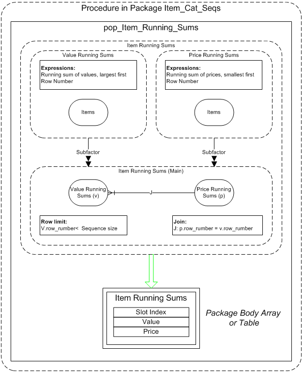
pop_Item_Running_Sums
Procedure that populates a temporary table, ITEM_RUNNING_SUMS, with running sums of item values, ordered by value descending, and prices, ordered by price ascending, with cardinality 1 less than sequence size. It copies the records into an array, g_items_running_sum_lis, either table or array can be read within the different query variants.
PROCEDURE pop_Item_Running_Sums IS
BEGIN
  DELETE item_running_sums;
  INSERT INTO item_running_sums
  WITH vals AS (
    SELECT ROWNUM rn, sum_value
      FROM (SELECT Sum(item_value) OVER (ORDER BY item_value DESC, id) sum_value
              FROM items
             ORDER BY item_value DESC, id)
  ), prices AS (
    SELECT ROWNUM rn, sum_price
      FROM (SELECT Sum(item_price) OVER (ORDER BY item_price, id) sum_price
              FROM items
             ORDER BY item_price, id)
  )
  SELECT v.rn, sum_value, sum_price
    FROM vals v
    JOIN prices p ON p.rn = v.rn
   WHERE v.rn < g_seq_size;

  SELECT slot_index, sum_value, sum_price
    BULK COLLECT INTO g_items_running_sum_lis
    FROM item_running_sums
   ORDER BY slot_index;
END pop_Item_Running_Sums;
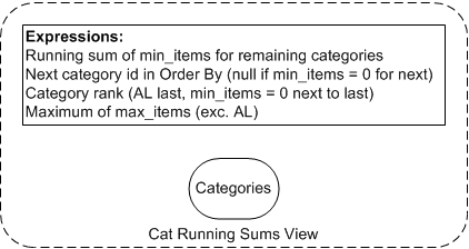
View CATEGORY_RSUMS_V
↑ Pre-calculation Procedures
This view has columns and analytic expressions based on the CATEGORIES table, and is used in the procedure pop_Items_Ranked. It’s been extracted into a view to allow re-use in some later variations on the procedure.
CREATE OR REPLACE VIEW category_rsums_v AS
    SELECT id, min_items, max_items,
           Sum(CASE WHEN id != 'AL' THEN min_items END)
             OVER (ORDER BY CASE WHEN min_items > 0 THEN max_items - min_items END DESC,
                            min_items,
                            max_items DESC,
                            id DESC)                      min_remain,
           Lead(CASE WHEN min_items > 0 THEN id END)
            OVER (ORDER BY CASE WHEN min_items > 0 THEN max_items - min_items END,
                           min_items DESC,
                           max_items,
                           id)                            next_cat_id,
           Row_Number()
                    OVER (ORDER BY CASE WHEN id = 'AL' THEN 2 ELSE 1 END,
                                   CASE WHEN min_items > 0 THEN max_items - min_items END,
                                   min_items DESC,
                                   max_items,
                                   id)                    cat_rnk,
           MAX(CASE WHEN id != 'AL' THEN max_items END) OVER () max_max_items
      FROM categories
     WHERE max_items > 0
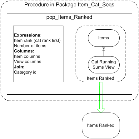
pop_Items_Ranked
Procedure that populates a temporary table, ITEMS_RANKED, with a set of item records with pre-calculated rank and other values.
PROCEDURE pop_Items_Ranked IS
BEGIN
  DELETE items_ranked;
  INSERT INTO items_ranked
  SELECT itm.id,
         itm.category_id,
         itm.item_price,
         itm.item_value,
         crs.min_items,
         crs.max_items,
         crs.min_remain,
         crs.next_cat_id,
         Row_Number() OVER (ORDER BY crs.cat_rnk, itm.item_value DESC, itm.id),
         Count(*) OVER ()
    FROM items itm
    JOIN category_rsums_v crs
      ON crs.id = itm.category_id;
END pop_Items_Ranked;
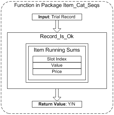
Query Where Function - Record_Is_Ok
This function is used in certain queries to contain constraint logic: It returns Y if the values from the current trial record passed in are deemed valid, based on a pre-calculated array, and optimization constraint logic.
FUNCTION Record_Is_Ok(
            p_lev                          PLS_INTEGER,
            p_tot_value                    PLS_INTEGER,
            p_tot_price                    PLS_INTEGER,
            p_cat_id                       VARCHAR2,
            p_cat_id_new                   VARCHAR2,
            p_same_cats                    VARCHAR2,
            p_next_cat_id                  VARCHAR2,
            p_min_items                    PLS_INTEGER,
            p_min_items_new                PLS_INTEGER,
            p_max_items_new                PLS_INTEGER,
            p_min_remain_new               PLS_INTEGER)
            RETURN                         VARCHAR2 IS
  l_test_value      PLS_INTEGER := p_tot_value;
  l_test_price      PLS_INTEGER := p_tot_price;
  l_slots_left      PLS_INTEGER := g_seq_size - p_lev - 1;
BEGIN

  IF l_slots_left > 0 THEN
    l_test_value := p_tot_value + g_items_running_sum_lis(l_slots_left).sum_value;
    l_test_price := p_tot_price + g_items_running_sum_lis(l_slots_left).sum_price;
  END IF;

  IF l_test_value >= g_min_value AND l_test_price <= g_max_price AND p_lev < g_seq_size AND
     CASE p_cat_id_new WHEN p_cat_id THEN p_same_cats + 1 ELSE 1 END <= p_max_items_new AND
     l_slots_left + Least(CASE p_cat_id_new WHEN p_cat_id THEN p_same_cats + 1 ELSE 1 END,
                          p_min_items_new) >= p_min_remain_new AND
     (p_cat_id_new = p_cat_id OR p_same_cats >= p_min_items) AND
     (p_cat_id_new = p_cat_id OR p_cat_id_new = Nvl(p_next_cat_id, p_cat_id_new)) THEN

    RETURN 'Y';
  ELSE
    RETURN 'N';
  END IF;

END Record_Is_Ok;
Recursive SQL with Temporary Tables
↑ 4 Recursive SQL with PL/SQL
↓ Results
↓ Query Structure
View: RSF_IRK_IRS_TABS_V
In this view, we replace the subqueries with temporary tables with records pre-populated.
Results
↑ Recursive SQL with Temporary Tables
| Code | View | IRK Access | IRS Access | IRK/TRW-Conditions | IRS/TRW-Conditions |
|---|---|---|---|---|---|
| SQL | RSF_SQL_V - original pure SQL recursive query | Subquery | Subquery | Inline | Inline |
| SQM | RSF_SQL_MATERIAL_V - pure SQL with a materialize hint | Subquery | Subquery | Inline | Inline |
| IIT | RSF_IRK_IRS_TABS_V - temporary tables for IRK and IRS | Table | Table | Inline | Inline |
Brazil
| KEEP_NUM | MIN_VALUE | Solution Set | SQL | SQM | IIT |
|---|---|---|---|---|---|
| 10 | 0 | B-B (suboptimal) | 0.7 | 0.3 | 0.1 |
| 100 | 0 | B-A (optimal) | 6.5 | 2.9 | 1.1 |
| 100 | 10748 | B-A (optimal) | 0.4 | 0.2 | 0.1 |
| 0 | 10748 | B-A (optimal) | 0.7 | 0.4 | 0.1 |
England
| KEEP_NUM | MIN_VALUE | Solution Set | SQL | SQM | IIT |
|---|---|---|---|---|---|
| 50 | 0 | E-B (suboptimal) | 208 | 52 | 9 |
| 300 | 0 | E-A (optimal) | 1253 | 318 | 72 |
| 300 | 1952 | E-A (optimal) | 80 | 20 | 3 |
| 0 | 1952 | E-A (optimal) | 2288 | 1727 | 214 |
We see that the new view is much faster than the pure SQL views in all cases.
Query Structure
↑ Recursive SQL with Temporary Tables
↓ Query SQL
↓ Execution Plan
Query SQL
WITH tree_walk(path_rnk, item_rnk, lev, tot_price, tot_value, cat_id, next_cat_id, same_cats, min_items, cats_path, path, seq_size) AS (
    SELECT 0, 0, 0, 0, 0, 'AL', cat_id, 0, 0, '','', To_Number(SYS_Context('RECURSION_CTX', 'SEQ_SIZE'))
      FROM items_ranked
     WHERE item_rnk = 1
     UNION ALL
    SELECT Row_Number() OVER (PARTITION BY trw.cats_path || irk.cat_id ORDER BY trw.tot_value + irk.item_value DESC),
           irk.item_rnk,
           trw.lev + 1,
           trw.tot_price + irk.item_price,
           trw.tot_value + irk.item_value,
           irk.cat_id,
           irk.next_cat_id,
           CASE irk.cat_id WHEN trw.cat_id THEN trw.same_cats + 1 ELSE 1 END,
           irk.min_items,
           trw.cats_path || irk.cat_id,
           trw.path || irk.item_id,
           trw.seq_size
      FROM tree_walk trw
      JOIN items_ranked irk
        ON irk.item_rnk BETWEEN (trw.item_rnk + 1) AND (irk.n_items - (trw.seq_size - trw.lev - 1))
      LEFT JOIN item_running_sums irs
        ON irs.slot_index = trw.seq_size - trw.lev - 1
     WHERE trw.tot_price + irk.item_price + Nvl(irs.sum_price, 0) <= To_Number(SYS_Context('RECURSION_CTX', 'MAX_PRICE'))
       AND trw.tot_value + irk.item_value + Nvl(irs.sum_value, 0) >= To_Number(SYS_Context('RECURSION_CTX', 'MIN_VALUE'))
       AND trw.lev < trw.seq_size
       AND CASE irk.cat_id WHEN trw.cat_id THEN trw.same_cats + 1 ELSE 1 END <= irk.max_items
       AND trw.seq_size - (trw.lev + 1) + Least(CASE irk.cat_id
                                              WHEN trw.cat_id THEN trw.same_cats + 1 ELSE 1 END,
                                              irk.min_items)
           >= irk.min_remain
       AND (irk.cat_id = trw.cat_id OR trw.same_cats >= trw.min_items)
       AND (irk.cat_id = trw.cat_id OR irk.cat_id = Nvl(trw.next_cat_id, irk.cat_id))
       AND (trw.path_rnk <= To_Number(SYS_Context('RECURSION_CTX', 'KEEP_NUM')) OR To_Number(Nvl(SYS_Context('RECURSION_CTX', 'KEEP_NUM'), '0')) = 0)
)
SELECT path,
       tot_value,
       tot_price,
       Row_Number() OVER (ORDER BY tot_value DESC, tot_price) rnk
  FROM tree_walk
 WHERE lev = seq_size
Execution Plan
Plan hash value: 3930817166
------------------------------------------------------------------------------------------------------------------------------------------------------------------------------------
| Id  | Operation                                    | Name               | Starts | E-Rows | A-Rows |   A-Time   | Buffers | Reads  | Writes |  OMem |  1Mem | Used-Mem | Used-Tmp|
------------------------------------------------------------------------------------------------------------------------------------------------------------------------------------
|   0 | SELECT STATEMENT                             |                    |      1 |        |     10 |00:03:34.01 |      47M|  89254 |  89254 |       |       |          |         |
|   1 |  SORT ORDER BY                               |                    |      1 |      2 |     10 |00:03:34.01 |      47M|  89254 |  89254 |  2048 |  2048 | 2048  (0)|         |
|*  2 |   VIEW                                       | RSF_IRK_IRS_TABS_V |      1 |      2 |     10 |00:03:34.01 |      47M|  89254 |  89254 |       |       |          |         |
|*  3 |    WINDOW SORT PUSHED RANK                   |                    |      1 |      2 |     10 |00:03:34.01 |      47M|  89254 |  89254 |  2048 |  2048 | 2048  (0)|         |
|*  4 |     VIEW                                     |                    |      1 |      2 |     50 |00:03:33.99 |      47M|  89254 |  89254 |       |       |          |         |
|   5 |      UNION ALL (RECURSIVE WITH) BREADTH FIRST|                    |      1 |        |   1842K|00:00:43.10 |      47M|  89254 |  89254 |    97M|  3375K|   97M (0)|         |
|*  6 |       INDEX UNIQUE SCAN                      | SYS_IOT_TOP_177213 |      1 |      1 |      1 |00:00:00.01 |       2 |      0 |      0 |       |       |          |         |
|   7 |       WINDOW SORT                            |                    |     12 |      1 |   1842K|00:02:53.85 |    1847K|  89254 |  78167 |   205M|  4802K|   97M (1)|     185M|
|   8 |        NESTED LOOPS                          |                    |     12 |      1 |   1842K|00:01:26.25 |    1847K|  18352 |   7265 |       |       |          |         |
|*  9 |         HASH JOIN OUTER                      |                    |     12 |      1 |   1842K|00:00:01.60 |       4 |  18352 |   7265 |   127M|  9325K|  152M (0)|      49M|
|  10 |          RECURSIVE WITH PUMP                 |                    |     12 |        |   1842K|00:00:00.47 |       1 |  11087 |      0 |       |       |          |         |
|  11 |          BUFFER SORT (REUSE)                 |                    |     11 |        |    110 |00:00:00.01 |       3 |      0 |      0 | 73728 | 73728 |          |         |
|  12 |           TABLE ACCESS FULL                  | ITEM_RUNNING_SUMS  |      1 |     10 |     10 |00:00:00.01 |       3 |      0 |      0 |       |       |          |         |
|* 13 |         INDEX RANGE SCAN                     | SYS_IOT_TOP_177213 |   1842K|      1 |   1842K|00:02:30.77 |    1847K|      0 |      0 |       |       |          |         |
------------------------------------------------------------------------------------------------------------------------------------------------------------------------------------
Predicate Information (identified by operation id):
---------------------------------------------------
2 - filter("RNK"<=:TOP_N)
3 - filter(ROW_NUMBER() OVER ( ORDER BY INTERNAL_FUNCTION("TOT_VALUE") DESC ,"TOT_PRICE")<=:TOP_N)
4 - filter("LEV"="SEQ_SIZE")
6 - access("ITEM_RNK"=1)
9 - access("IRS"."SLOT_INDEX"="TRW"."SEQ_SIZE"-"TRW"."LEV"-1)
13 - access("IRK"."ITEM_RNK">="TRW"."ITEM_RNK"+1)
filter(("IRK"."ITEM_RNK"<="IRK"."N_ITEMS"-("TRW"."SEQ_SIZE"-"TRW"."LEV"-1) AND "IRK"."MAX_ITEMS">=CASE "IRK"."CAT_ID" WHEN "TRW"."CAT_ID" THEN "TRW"."SAME_CATS"+1
ELSE 1 END  AND "TRW"."TOT_PRICE"+"IRK"."ITEM_PRICE"+NVL("IRS"."SUM_PRICE",0)<=TO_NUMBER(SYS_CONTEXT('RECURSION_CTX','MAX_PRICE')) AND
"TRW"."TOT_VALUE"+"IRK"."ITEM_VALUE"+NVL("IRS"."SUM_VALUE",0)>=TO_NUMBER(SYS_CONTEXT('RECURSION_CTX','MIN_VALUE')) AND
"IRK"."MIN_REMAIN"<="TRW"."SEQ_SIZE"-("TRW"."LEV"+1)+LEAST(CASE "IRK"."CAT_ID" WHEN "TRW"."CAT_ID" THEN "TRW"."SAME_CATS"+1 ELSE 1 END ,"IRK"."MIN_ITEMS") AND
("IRK"."CAT_ID"="TRW"."CAT_ID" OR "TRW"."SAME_CATS">="TRW"."MIN_ITEMS") AND ("IRK"."CAT_ID"="TRW"."CAT_ID" OR "IRK"."CAT_ID"=NVL("TRW"."NEXT_CAT_ID","IRK"."CAT_ID"))))
Note
-----
- dynamic statistics used: dynamic sampling (level=2)
- statistics feedback used for this statement
Notice that in step 13 IRK is accessed via the INDEX RANGE SCAN operation, without any second table access, since the table is index organized.
Recursive SQL with Temporary Table and Where Function
↑ 4 Recursive SQL with PL/SQL
↓ Results
↓ Query Structure
↓ Execution Plan
View: RSF_IRK_TAB_WHERE_FUN_V
Having got good improvements from replacing the three initial subqueries with two pre-computed temporary tables, we now investigate whether using a function in the WHERE clause could simplify and/or improve the performance of the query further. This approach allows us to avoid joining the second table, ITEM_RUNNING_SUMS, in the query itself, instead accessing the corresponding array within a function used to validate the current trial record.
We will start by reporting the results, before describing it in more detail with execution plan in subsequent sections.
Results
↑ Recursive SQL with Temporary Table and Where Function
Note: IRK, IRS and TRW in the table below refer to the temporary tables/arrays for ITEMS_RANKED and ITEM_RUNNING_SUMS, and the recursive subquery respectively.
| Code | View | IRK Access | IRS Access | IRK/TRW-Conditions | IRS/TRW-Conditions |
|---|---|---|---|---|---|
| SQL | RSF_SQL_V - original pure SQL recursive query | Subquery | Subquery | Inline | Inline |
| SQM | RSF_SQL_MATERIAL_V - pure SQL with a materialize hint | Subquery | Subquery | Inline | Inline |
| IIT | RSF_IRK_IRS_TABS_V - temporary tables for IRK and IRS | Table | Table | Inline | Inline |
| ITW | RSF_IRK_TAB_WHERE_FUN_V - temporary table for IRK, with function accessing IRS array in WHERE clause | Table | Record_Is_Ok | Record_Is_Ok | Record_Is_Ok |
Brazil
| KEEP_NUM | MIN_VALUE | Solution Set | SQL | SQM | IIT | ITW |
|---|---|---|---|---|---|---|
| 10 | 0 | B-B (suboptimal) | 0.7 | 0.3 | 0.1 | 0.2 |
| 100 | 0 | B-A (optimal) | 6.5 | 2.9 | 1.1 | 1.6 |
| 100 | 10748 | B-A (optimal) | 0.4 | 0.2 | 0.1 | 0.2 |
| 0 | 10748 | B-A (optimal) | 0.7 | 0.4 | 0.1 | 0.5 |
England
| KEEP_NUM | MIN_VALUE | Solution Set | SQL | SQM | IIT | ITW |
|---|---|---|---|---|---|---|
| 50 | 0 | E-B (suboptimal) | 208 | 52 | 9 | 11 |
| 300 | 0 | E-A (optimal) | 1253 | 318 | 72 | 82 |
| 300 | 1952 | E-A (optimal) | 80 | 20 | 3 | 8 |
| 0 | 1952 | E-A (optimal) | 2288 | 1727 | 214 | 1181 |
We see that the new view, ITW, like the previous one, IIT, when compared with SQM, gives much improved performance on the England dataset, but is much slower than IIT in two cases.
One might surmise that the poor result on the final pair, where much more work is being done, may be at least partly due to context switching between SQL amd PL/SQL when invoking the function in the Where clause (Item_Cat_Seqs.Record_Is_Ok, see below). This phenomenon is discussed in an old AskTom thread, Context Switch, from which I extract:
There is a call overhead to go from SQL to PLSQL (the “hit” is most evident when SQL invokes PLSQL - not so much the other way, when SQL is embedded in PLSQL). Even if this hit is very very small (say 1/1000th of a second) - if you do it enough, it adds up. So, if it can be avoided - it should be.
It can be difficult to assess the impact of context switching in isolation because the execution plans may differ between view versions, and also because the execution plans do not reveal all relevant information. We’ll look at this in more detail in the next main section, Impact of Context Switching.
Query Structure
↑ Recursive SQL with Temporary Table and Where Function
The following query removes the join to ITEM_RUNNING_SUMS, by use of a function call in the WHERE clause, in the package Item_Cat_Seqs:
- Record_Is_Ok: Scalar function that returns Y if the values from the current trial record passed in are deemed valid, based on pre-calculated arrays
WITH tree_walk(path_rnk, item_rnk, lev, tot_price, tot_value, cat_id, next_cat_id, same_cats, min_items, cats_path, path, seq_size) AS (
    SELECT 0, 0, 0, 0, 0, 'AL', cat_id, 0, 0, '','', To_Number(SYS_Context('RECURSION_CTX', 'SEQ_SIZE'))
      FROM items_ranked
     WHERE item_rnk = 1
     UNION ALL
    SELECT Row_Number() OVER (PARTITION BY trw.cats_path || irk.cat_id ORDER BY trw.tot_value + irk.item_value DESC),
           irk.item_rnk,
           trw.lev + 1,
           trw.tot_price + irk.item_price,
           trw.tot_value + irk.item_value,
           irk.cat_id,
           irk.next_cat_id,
           CASE irk.cat_id WHEN trw.cat_id THEN trw.same_cats + 1 ELSE 1 END,
           irk.min_items,
           trw.cats_path || irk.cat_id,
           trw.path || irk.item_id,
           trw.seq_size
      FROM tree_walk trw
      JOIN items_ranked irk
        ON irk.item_rnk BETWEEN (trw.item_rnk + 1) AND (irk.n_items - (trw.seq_size - trw.lev - 1))
     WHERE Item_Cat_Seqs.Record_Is_Ok(p_lev             => trw.lev,
                                      p_tot_value       => trw.tot_value + irk.item_value,
                                      p_tot_price       => trw.tot_price + irk.item_price,
                                      p_cat_id          => trw.cat_id,
                                      p_cat_id_new      => irk.cat_id,
                                      p_same_cats       => trw.same_cats,
                                      p_next_cat_id     => trw.next_cat_id,
                                      p_min_items       => trw.min_items,
                                      p_min_items_new   => irk.min_items,
                                      p_max_items_new   => irk.max_items,
                                      p_min_remain_new  => irk.min_remain) = 'Y'
            AND (trw.path_rnk <= To_Number(SYS_Context('RECURSION_CTX', 'KEEP_NUM')) OR To_Number(Nvl(SYS_Context('RECURSION_CTX', 'KEEP_NUM'), '0')) = 0)
)
SELECT path,
       tot_value,
       tot_price,
       Row_Number() OVER (ORDER BY tot_value DESC, tot_price) rnk
  FROM tree_walk
 WHERE lev = seq_size
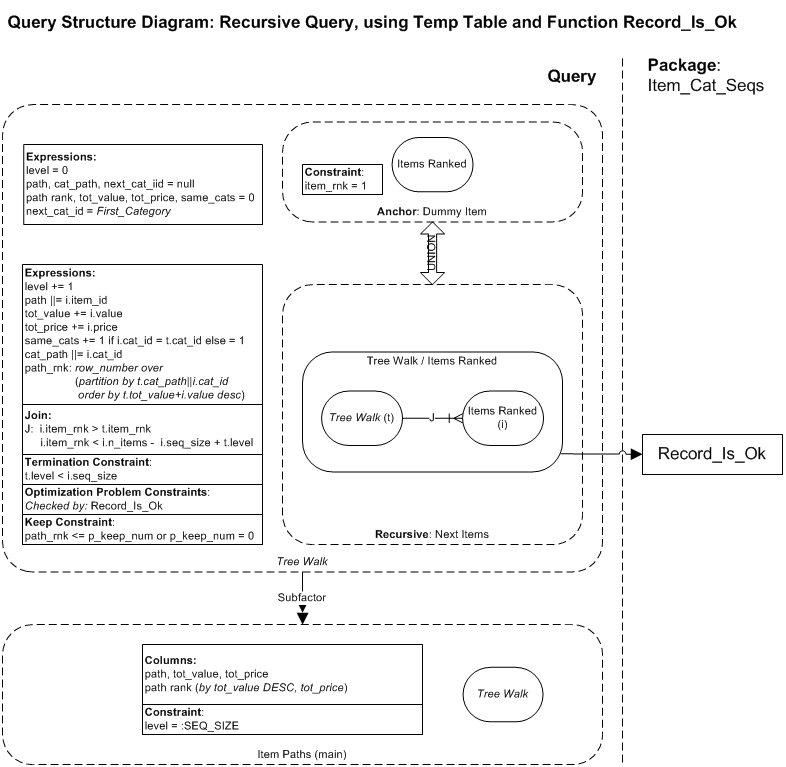
Execution Plan
↑ Recursive SQL with Temporary Table and Where Function
The execution plan for the query is as follows (England dataset, KEEP_NUM = 0, MIN_VALUE = 1952):
Plan hash value: 57043923
-----------------------------------------------------------------------------------------------------------------------------------------------------------------------------------------
| Id  | Operation                                    | Name                    | Starts | E-Rows | A-Rows |   A-Time   | Buffers | Reads  | Writes |  OMem |  1Mem | Used-Mem | Used-Tmp|
-----------------------------------------------------------------------------------------------------------------------------------------------------------------------------------------
|   0 | SELECT STATEMENT                             |                         |      1 |        |     10 |00:09:41.87 |      47M|  54062 |  54062 |       |       |          |         |
|   1 |  SORT ORDER BY                               |                         |      1 |      2 |     10 |00:09:41.87 |      47M|  54062 |  54062 |  2048 |  2048 | 2048  (0)|         |
|*  2 |   VIEW                                       | RSF_IRK_TAB_WHERE_FUN_V |      1 |      2 |     10 |00:09:41.87 |      47M|  54062 |  54062 |       |       |          |         |
|*  3 |    WINDOW SORT PUSHED RANK                   |                         |      1 |      2 |     10 |00:09:41.87 |      47M|  54062 |  54062 |  2048 |  2048 | 2048  (0)|         |
|*  4 |     VIEW                                     |                         |      1 |      2 |     50 |00:09:41.83 |      47M|  54062 |  54062 |       |       |          |         |
|   5 |      UNION ALL (RECURSIVE WITH) BREADTH FIRST|                         |      1 |        |   1842K|00:00:43.57 |      47M|  54062 |  54062 |    97M|  3375K|   97M (0)|         |
|*  6 |       INDEX UNIQUE SCAN                      | SYS_IOT_TOP_177213      |      1 |      1 |      1 |00:00:00.01 |       2 |      0 |      0 |       |       |          |         |
|   7 |       WINDOW SORT                            |                         |     12 |      1 |   1842K|00:15:41.55 |    1847K|  54062 |  42975 |   188M|  4610K|   97M (1)|     169M|
|   8 |        NESTED LOOPS                          |                         |     12 |      1 |   1842K|00:09:08.37 |    1847K|  11087 |      0 |       |       |          |         |
|   9 |         RECURSIVE WITH PUMP                  |                         |     12 |        |   1842K|00:00:00.73 |       1 |  11087 |      0 |       |       |          |         |
|* 10 |         INDEX RANGE SCAN                     | SYS_IOT_TOP_177213      |   1842K|      1 |   1842K|00:17:08.52 |    1847K|      0 |      0 |       |       |          |         |
-----------------------------------------------------------------------------------------------------------------------------------------------------------------------------------------
Predicate Information (identified by operation id):
---------------------------------------------------
2 - filter("RNK"<=:TOP_N)
3 - filter(ROW_NUMBER() OVER ( ORDER BY INTERNAL_FUNCTION("TOT_VALUE") DESC ,"TOT_PRICE")<=:TOP_N)
4 - filter("LEV"="SEQ_SIZE")
6 - access("ITEM_RNK"=1)
10 - access("IRK"."ITEM_RNK">="TRW"."ITEM_RNK"+1)
filter(("IRK"."ITEM_RNK"<="IRK"."N_ITEMS"-("TRW"."SEQ_SIZE"-"TRW"."LEV"-1) AND "ITEM_CAT_SEQS"."RECORD_IS_OK"(INTERNAL_FUNCTION("TRW"."LEV"),"TRW"."TOT_VALUE"+"IRK"."ITEM
_VALUE","TRW"."TOT_PRICE"+"IRK"."ITEM_PRICE","TRW"."CAT_ID","IRK"."CAT_ID",TO_CHAR("TRW"."SAME_CATS"),"TRW"."NEXT_CAT_ID",INTERNAL_FUNCTION("TRW"."MIN_ITEMS"),INTERNAL_FUNCTION(
"IRK"."MIN_ITEMS"),INTERNAL_FUNCTION("IRK"."MAX_ITEMS"),INTERNAL_FUNCTION("IRK"."MIN_REMAIN"))='Y'))
Note
-----
- dynamic statistics used: dynamic sampling (level=2)
- statistics feedback used for this statement
We see that the execution plan is slightly simpler than the previous plan, with the IRS array reference now inside the new function. This means that, where the driving row set for the nested loops join previously was the result of a hash join between the recursive subquery and ITEM_RUNNING_SUMS:
|*  9 |         HASH JOIN OUTER                      |                    |
|  10 |          RECURSIVE WITH PUMP                 |                    |
|  11 |          BUFFER SORT (REUSE)                 |                    |
|  12 |           TABLE ACCESS FULL                  | ITEM_RUNNING_SUMS  |
we now just have the recursive subquery in step 9.
The A-Rows for all comparable steps are identical, as are the Buffers, and the Reads, Writes and memory uses are all either the same, or smaller in the current plan. This raises an obvious question: Why does the query take 5 times as much time to execute as the earlier one without the WHERE clause function? Could it be down to context switching? We cannot tell from the plan how much overhead is added due to context switching, and we’ll investigate that issue in the next section.
Impact of Context Switching
↑ 4 Recursive SQL with PL/SQL
↓ Counting Function Calls
↓ Function Code
↓ Timer Set Results
In the last section we noted that the view with the IRS array reference and associated conditions inside a new function performed much more slowly than the previous view with these explicitly within the query. We also saw that the A-Rows value for the inner INDEX RANGE SCAN against the ITEMS_RANKED index-organized table was the same in both cases at 1842K (steps 13 and 10, respectively). However, it is important to understand that the A-Rows value is the number of records returned once the filter conditions have been applied, including the condition that the Record_Is_Ok function returns ‘Y’, and does not reflect the number of function calls made.
Counting Function Calls
For this reason, to better understand what’s going on we have created a second version of the function, Record_Is_Ok_TS, and the view, RSF_IRK_TAB_WHERE_FUN_TS_V, with code timing added within the function. We have also added a parameter, p_do_timing, to the Init function defaulting to FALSE, and when TRUE the function now creates a new timer set with its handle stored in a package global, g_timer_set. The call before querying the view is then:
BEGIN
  Item_Cat_Seqs.Init(p_keep_num      => &KEEP_NUM,
                     p_min_value     => &MIN_VALUE,
                     p_do_timing     => TRUE);
END;
with timer set creation logic added:
  IF p_do_timing THEN
    g_timer_set := Timer_Set.Construct ('Init, KEEP_NUM-MIN_VALUE: ' || p_keep_num || '-' || p_min_value);
  ELSE
    g_timer_set := NULL;
  END IF;
The timer set result is printed after the query using a new procedure, Write_Init_Timer_Set.
EXEC Item_Cat_Seqs.Write_Init_Timer_Set;
The timer sets has calls to Increment_Time before both ‘Y’ and ‘N’ returns, measuring them separately. The revised function is shown below.
Function Code
FUNCTION Record_Is_Ok_TS(
            p_lev                          PLS_INTEGER,
            p_tot_value                    PLS_INTEGER,
            p_tot_price                    PLS_INTEGER,
            p_cat_id                       VARCHAR2,
            p_cat_id_new                   VARCHAR2,
            p_same_cats                    VARCHAR2,
            p_next_cat_id                  VARCHAR2,
            p_min_items                    PLS_INTEGER,
            p_min_items_new                PLS_INTEGER,
            p_max_items_new                PLS_INTEGER,
            p_min_remain_new               PLS_INTEGER)
            RETURN                         VARCHAR2 IS
  l_test_value      PLS_INTEGER := p_tot_value;
  l_test_price      PLS_INTEGER := p_tot_price;
  l_slots_left      PLS_INTEGER := g_seq_size - p_lev - 1;
BEGIN
  IF l_slots_left > 0 THEN
    l_test_value := p_tot_value + g_items_running_sum_lis(l_slots_left).sum_value;
    l_test_price := p_tot_price + g_items_running_sum_lis(l_slots_left).sum_price;
  END IF;
  IF l_test_value >= g_min_value AND l_test_price <= g_max_price AND p_lev < g_seq_size AND
     CASE p_cat_id_new WHEN p_cat_id THEN p_same_cats + 1 ELSE 1 END <= p_max_items_new AND
     l_slots_left + Least(CASE p_cat_id_new WHEN p_cat_id THEN p_same_cats + 1 ELSE 1 END,
                          p_min_items_new) >= p_min_remain_new AND
     (p_cat_id_new = p_cat_id OR p_same_cats >= p_min_items) AND
     (p_cat_id_new = p_cat_id OR p_cat_id_new = Nvl(p_next_cat_id, p_cat_id_new)) THEN
    Timer_Set.Increment_Time(g_timer_set, 'Record_Is_Ok - Y');
    RETURN 'Y';
  ELSE
    Timer_Set.Increment_Time(g_timer_set, 'Record_Is_Ok - N');
   RETURN 'N';
  END IF;
END Record_Is_Ok_TS;
Timer Set Results
Timer Set: Init, KEEP_NUM-MIN_VALUE: 0-1952, Constructed at 11 Jun 2024 01:39:17, written at 03:15:52
=====================================================================================================
Timer                Elapsed         CPU       Calls       Ela/Call       CPU/Call
----------------  ----------  ----------  ----------  -------------  -------------
init_Common             0.00        0.00           1        0.00200        0.00000
pop_Items_Ranked        0.01        0.00           1        0.00700        0.00000
Record_Is_Ok - Y       54.13       51.19     1842891        0.00003        0.00003
Record_Is_Ok - N     5741.37     5694.33   410655010        0.00001        0.00001
(Other)                 0.03        0.01           1        0.03000        0.01000
----------------  ----------  ----------  ----------  -------------  -------------
Total                5795.54     5745.53   412497904        0.00001        0.00001
----------------  ----------  ----------  ----------  -------------  -------------
[Timer timed (per call in ms): Elapsed: 0.01053, CPU: 0.01158]
The elapsed time in the original view without the code timing was 1181 seconds for the England dataset (KEEP_NUM = 0, MIN_VALUE = 1952), and this has increased dramatically to a total of 5,796 seconds, due to the impact of the code timing calls themselves. We are interested in the numbers of calls rather than the distorted timings.
There were 1,842,891 calls returning ‘Y’ and 410,655,010 returning ‘N’. The first figure corresponds to the A-Rows value of 1842K, while the ‘N’ calls result in the candidate record being filtered out.
This gives us some insight into why the time went from 214 seconds for IIT to 1181 seconds for ITW, despite fairly similar execution plans: A very large number of function calls were made to filter the rows. If we divide the difference in time by the total number of calls, we get:
Seconds per call = (1181 - 214 = 967) / (1842891 + 410655010 = 412497901) = 0.0000023 = 2.3E-6
By comparison the estimated overhead for a timing call is 1E-5, four times greater. The estimate is not very accurate, but we can see that a very small context switching overhead repeated many times has made a big impact on the time taken.
5 Conclusion
↑ Contents
↓ Results
↓ Lessons Learned
In this article, we used two larger test datasets to analyse the performance of the initial recursive query, with Value Filtering techniques included, as described in the fourth article, and looked at variations on the query designed to improve performance.
To conclude, we will summarise the results for the four recursive subquery views developed, then note some lessons learned.
Results
Note: IRK, IRS and TRW in the table below refer to the table/array for items ranked and item running sums, and the recursive subquery respectively.
| Code | View | IRK Access | IRS Access | IRK/TRW-Conditions | IRS/TRW-Conditions |
|---|---|---|---|---|---|
| SQL | RSF_SQL_V - original pure SQL recursive query | Subquery | Subquery | Inline | Inline |
| SQM | RSF_SQL_MATERIAL_V - pure SQL with a materialize hint | Subquery | Subquery | Inline | Inline |
| IIT | RSF_IRK_IRS_TABS_V - temporary tables for IRK and IRS | Table | Table | Inline | Inline |
| ITW | RSF_IRK_TAB_WHERE_FUN_V - temporary table for IRK, with function accessing IRS array in WHERE clause | Table | Record_Is_Ok | Record_Is_Ok | Record_Is_Ok |
Brazil
| KEEP_NUM | MIN_VALUE | Solution Set | SQL | SQM | IIT | ITW |
|---|---|---|---|---|---|---|
| 0 | 0 | ORA-01652: unable to extend temp segment by 128 in tablespace TEMP | NA | NA | NA | NA |
| 10 | 0 | B-B (suboptimal) | 0.7 | 0.3 | 0.1 | 0.2 |
| 100 | 0 | B-A (optimal) | 6.5 | 2.9 | 1.1 | 1.6 |
| 100 | 10748 | B-A (optimal) | 0.4 | 0.2 | 0.1 | 0.2 |
| 0 | 10748 | B-A (optimal) | 0.7 | 0.4 | 0.1 | 0.5 |
England
| KEEP_NUM | MIN_VALUE | Solution Set | SQL | SQM | IIT | ITW |
|---|---|---|---|---|---|---|
| 0 | 0 | ORA-01652: unable to extend temp segment by 128 in tablespace TEMP | NA | NA | NA | NA |
| 50 | 0 | E-B (suboptimal) | 208 | 52 | 9 | 11 |
| 300 | 0 | E-A (optimal) | 1253 | 318 | 72 | 82 |
| 300 | 1952 | E-A (optimal) | 80 | 20 | 3 | 8 |
| 0 | 1952 | E-A (optimal) | 2288 | 1727 | 214 | 1181 |
Lessons Learned
We can summarise the principle points we have learned in relation to solving these problems using recursive queries:
- Even when truncating subsequences as soon as possible, recursive subqueries for these datasets fail to complete until we introduce non-zero values for at least one of the
Value Filteringparameters - Oracle does not by default materialize subquery factors that are referenced only in recursive subqueries, and this can adversely affect performance
- A materialize hint can improve performance, but we found that extracting the subquery factors into temporary tables was better still
- On the hardest dataset / parameter pair problem the temporary table IIT solution method was 10x faster than pure SQL
- Putting query WHERE conditions inside a PL/SQL function may result in considerable adverse performance impacts
- The performance impact depends on how many times the function is called, and this can be difficult to determine, since the execution plans do not report this information
- Using a known minimum value to truncate solution paths,
Value Bound Filtering, can improve performance considerably, without loss of optimality - Using
Value Rank Filteringto retain only the best subsequences by category path can improve performance considerably, although it may involve loss of optimality
In the next article we will demonstrate how PL/SQL can be used to implement both recursive and iterative versions of the basic algorithm with embedded SQL, and we’ll go on to implement an Iterative Refinement algorithm that will prove to be highly efficient.