Shortest Path Analysis of Large Networks by SQL and PL/SQL
This article is on the use of SQL and PL/SQL to solve shortest path network problems on an Oracle database. It provides solutions in pure SQL (based on previous articles by the author), and solutions in PL/SQL with embedded SQL that scale better for larger problems.
It applies the solutions to a range of problems, upto a size of 2,800,309 nodes and 109,262,592 links.
Standard and custom methods for execution time profiling of the code are included, and one of the algorithms implemented in PL/SQL is tuned based on the profiling.
The two PL/SQL entry points have automated unit tests using the Math Function Unit Testing design pattern, Trapit - Oracle PL/SQL unit testing module.
All code and examples are available on GitHub.
Movie Morsel: Six Degrees of Kevin Bacon
There is a series of mp4 recordings, in the mp4 folder on GitHub, briefly going through the sections of the blog post, which can also be viewed via Twitter:
| Recording | Tweet |
|---|---|
| sps_1_overview.mp4 | 1: Overview |
| sps_2_shortest_path_problems.mp4 | 2: Shortest Path Problems |
| sps_3_two_algorithms.mp4 | 3: Two Algorithms |
| sps_4_example_datasets.mp4 | 4: Example Datasets |
| sps_5_data_model.mp4 | 5: Data Model |
| sps_6_network_paths_by_sql.mp4 | 6: Network Paths by SQL |
| sps_7_min_pathfinder.mp4 | 7: Min Pathfinder |
| sps_8_subnet_grouper.mp4 | 8: Subnetwork Grouper |
| sps_9_code_timing_subnet_grouper.mp4 | 9: Code Timing Subnet Grouper |
| sps_10_profiling.mp4 | 10: Oracle Profilers |
| sps_11_tuning_1_isolated_nodes.mp4 | 11: Tuning 1, Isolated Nodes |
| sps_12_tuning_2_isolated_links.mp4 | 12: Tuning 2, Isolated Links |
| sps_13_tuning_3_root_selector.mp4 | 13: Tuning 3, Root Node Selector |
| sps_14_unit_testing.mp4 | 14: Unit Testing |
There is also a presentation, given in Dublin on 5 September 2022 for the 2022 Oracle User Group conference (the .pptx file is in the GitHub root folder):
Contents
↓ Background
↓ Shortest Path Problems
↓ Two Algorithms
↓ Example Datasets
↓ Data Model
↓ Network Paths by SQL
↓ Min Pathfinder
↓ Subnetwork Grouper
↓ Tuning Subnetwork Grouper
↓ Unit Testing
↓ Conclusion
↓ References
Background
In 2015 I posted a number of articles on network analysis via SQL and array-based PL/SQL, including SQL for Shortest Path Problems 2: A Branch and Bound Approach and PL/SQL Pipelined Function for Network Analysis. These were tested on networks up to a size of 58,228 nodes and 214,078 links, but were not intended for really large networks.
Recently, I came across (by way of an article on using PostgreSQL for network analysis, Using the PostgreSQL Recursive CTE - Part Two, Bryn Llewellyn, March 2021) a set of network datasets published by an American college, Bacon Numbers Datasets from Oberlin College, December 2016. These range in size up to 2,800,309 nodes and 109,262,592 links, and I wondered if I could develop my ideas further to enable solution in Oracle SQL and PL/SQL of the larger networks.
Shortest Path Problems
↑ Contents
↓ Network Paths
↓ Min Pathfinder Problem
↓ Subnetwork Grouper Problem
Shortest path problems entail finding the minimum number of nodes between a given root node and any or all other nodes in a network. We will consider undirected networks described by links consisting of pairs of nodes, and the core problem will be that of finding the minimum length paths to all connected nodes from a given root node. Each link consisting of a pair of nodes will be unique (and if necessary we will de-duplicate in advance). Self-joining links that connect a node with itself cannot appear in a shortest path, so will be discarded in advance where necessary.
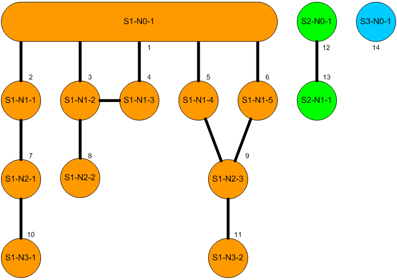
The diagram shows a network consisting of three connected subnetworks that we’ll use to illustrate the problems considered.
Network Paths
In a network with loops we can have paths of infinite length simply by repeating the loop paths. However, we will consider only acyclic paths, defined as paths without repetition of a node. For the main subnetwork above, we can show all possible acyclic paths from the root node S1-N0-1 by the arrows in the diagram:
Node      Path         Length
--------- ------------ ------
S1-N0-1   1                 0
S1-N1-1   ..2               1
S1-N2-1   ....7             2
S1-N3-1   ......10          3
S1-N1-2   ..3               1
S1-N1-3   ....4             2
S1-N2-2   ....8             2
S1-N1-3   ..4               1
S1-N1-2   ....3             2
S1-N2-2   ......8           3
S1-N1-4   ..5               1
S1-N2-3   ....9             2
S1-N1-5   ......6           3
S1-N3-2   ......11          3
S1-N1-5   ..6               1
S1-N2-3   ....9             2
S1-N1-4   ......5           3
S1-N3-2   ......11          3
In a looped network such as this one, some nodes can be reached by different paths. For example, the node, S1-N1-2 (numbered 3) can be reached in 1 step directly from the root, or in 2 steps via the node S1-N1-3.
Min Pathfinder Problem
↑ Shortest Path Problems
↓ Spanning Trees
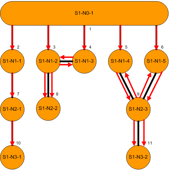
This is the main shortest path problem: We want to assign to each node a minimum path length from a given root node, and also a single path to each node consisting of a sequence of nodes that achieves the minimum length.
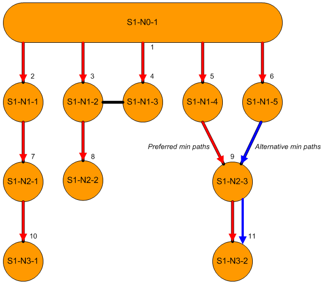
In a looped network we may have more than one path of shortest length. For example, in the diagram above we can reach nodes S1-N2-3 and S1-N3-2 in paths of length 3, via either S1-N1-4 or S1-N1-5. In such cases, we can rank the paths and choose a preferred path, for example by ranking the nodes prior to S1-N2-3 alphabetically.
Spanning Trees
In any connected network we can identify a spanning tree consisting of a set of links that includes all nodes and contains no loops. The minimum length paths for a subnetwork correspond to spanning trees, with the red links representing the preferred one of two in the diagram above, based on the stated alphabetical prior node ranking.
Subnetwork Grouper Problem
This problem is, given a network, split the nodes into their connected subnetworks. In the example diagram above there are three distinct subnetworks. We will identify the grouped nodes by assigning a single root node to each node in the subnetwork. This problem can be solved using a Min Pathfinder algorithm as a function called within a higher level algorithm.
Two Algorithms
↑ Contents
↓ Min Pathfinder Algorithm
↓ Subnetwork Grouper Algorithm
We have two main algorithms in relation to shortest path problems. The first, core, algorithm starts from an input root node and determines, for each connected node, the minimum length of path through the links from the root to the node, and also obtains a single sequence (‘path’) of nodes between the two. These paths constitute a spanning tree network of links from the root node to all connected nodes without loops, which can easily be traversed by a simple recursive procedure.
The second algorithm iterates over nodes using the first algorithm to obtain all nodes connected to a sequence of root nodes, assigning each connected node to its root node with its minimum path length. It iterates over currently unassigned nodes until all nodes are assigned to a root, and thus groups the nodes into connected subnetworks.
The algorithms are implemented in SQL and PL/SQL, but will first be described, and proven to work, in abstract terms.
Let N be the set of nodes {n}, and L be the set of links {l}, where each link l is a pair of nodes (nf, nt). The links are considered to be undirected.
Min Pathfinder Algorithm
↑ Two Algorithms
↓ Generating Minimum Length Path Node Sets
↓ Generating All Minimum Length Paths
↓ Generating A Single Minimum Length Path Per Node
↓ Shortest Paths and Spanning Trees
Generating Minimum Length Path Node Sets
Let k be an iteration number, starting with k = 0, which will correspond to an input root node, r say.
Let nk denote a node, n, reachable in a minimum of k steps from the root node, and let {nk} denote the set of all such nodes. In a tree network (i.e. a network without loops), there is a single path from the root to any other reachable node. If the network has loops then there may be multiple paths between nodes.
We might write the set of all nodes reachable in a minimum of k steps from the root node, r, as:
Nk(r) = {nk}(r)
Consider the set of all nodes that have a link connecting them to a node in Ni(r), but which are not themselves in any of the sets Nk(r) for k = 0,…,i. We can write this symbolically (dropping the (r) for concision), where N and L are the complete node and link sets respectively:

The union represents the fact that the new node may be at either end of the link, and note that a node in the set Ni+1 may occur in multiple links from the set Ni, but only appears once in the node set since set elements are unique.
Now we need to show that under our method of construction, Ni+1 matches our definition of Nk in general. This requires the following conditions to hold:
- All nodes in Ni+1 are reachable in i + 1 steps
This follows from the fact that the nodes are obtained as a single step from nodes reachable by definition in i steps - All nodes in Ni+1 are not reachable in < i + 1 steps
This follows from the fact that by definition Nk contains all nodes reachable in k steps where k < i + 1, and by construction Ni+1 excludes these nodes - No nodes not in Ni+1 are reachable in i + 1 steps
Any node reachable in i + 1 steps must be linked to a node reachable in i steps, which must by definition be in Ni, and by construction this would lead to the inclusion of the node reachable in i + 1 steps in Ni+1
Given that we know that the root node is reachable in zero steps, we have:
N0 = {r}
It follows, by induction, that the recursive definition of Ni+1 from Ni allows us to generate Nk for all k > 0.
Generating All Minimum Length Paths
A path, p, to a node, n, is a sequence of nodes starting from the root node with each adjacent pair of nodes appearing in the link set L.
We showed how to generate all the node sets reachable from a root node in a minimum number of steps. The generation process obtains the (i + 1)’th set by taking all the nodes linked to the i’th set and not in a prior set. We can extend this process to generate also all the minimum length paths associated with the nodes, by adding on these linked nodes to the prior paths. This can be expressed thus:

where (p, n) means the path obtained by adding the new node n onto the prior path in Pi, and Pk represents the set of all paths of length k that are minimum length paths to a node reachable from the root node, r.
P0 = {}
It’s easy to see how this allows us to generate Pk for all k > 0 in the same way as the iteration scheme for the node sets, Nk.
Generating A Single Minimum Length Path Per Node
We have seen how to generate all the minimum length paths to each node, but suppose we want to keep just one path for each node. We can do this by using a ranking function that uniquely ranks all minimum length paths to a node, say R(pi, ni) for each minimum length i, with:
R(p*i, ni) = 1 for a single path to node ni
Then we can write the iteration scheme for the set of optimal minimum length paths of length i + 1, P*i+1 based on those of length i thus:

P*0 = {}
Note that this guarantees that each node will have a single minimum length path generated, and also that any sub-path to a node generated as part of a path to a higher level node will be the same as the original path.
Shortest Paths and Spanning Trees
It is clear that the network comprised by the single minimum length paths to each node constitutes a spanning tree for the subnetwork connected to the root, i.e. a network connecting all the subnetwork nodes without loops.
It is important for efficient implementation to note that the tree network can be described by (node/prior node) links, so that each node does not need to have an explicit list of each node in its path, only the prior node.
Subnetwork Grouper Algorithm
Any undirected network can be partitioned into subsets in which each node in a subnetwork is reachable from any other node in the same subnetwork, but not from any other node. With N and L representing the full sets of nodes and links, we could write the sets of partitioning subsets NP and LP, say, in terms of the node and link subsets Ni and Li, respectively:


The sets are unique for the given network and of course the set cardinalities are the same:

Now let us see how we can generate the node subsets recursively. Suppose that we have the first i node subsets:

and let us write the set of all nodes not in the first i subsets thus:

and suppose that we have a ranking function defined on a node and node set pair, R(n, {n}), with:
R(n*, {n}) = 1 for a single node n* in {n}
Now, assuming we know how to generate the complete connected subnetwork, N(r), for any given root, r, as discussed in the first section above, we can generate the next node subset thus:

Example Datasets
↑ Contents
↓ 3 Subnetworks
↓ Foreign Keys
↓ Brightkite
↓ Bacon Numbers
We apply the algorithms to a range of network datasets. The first two small datasets comprise a made-up example, and a foreign key network from an Oracle database. The brightkite dataset represents a social network and comes from a university web site, and there are several datasets of varying sizes from another university web site representing actors’ appearances in films. Further details are given below.
| Dataset | #Nodes | #Links | #Subnetworks | #Isolated Nodes | #Isolated Links | Maxlev |
|---|---|---|---|---|---|---|
| three_subnets | 14 | 13 | 3 | 1 | 1 | 3 |
| foreign_keys | 289 | 319 | 43 | 0 | 19 | 8 |
| brightkite | 58,228 | 214,078 | 547 | 0 | 362 | 10 |
| bacon/small | 161 | 3,342 | 1 | 0 | 0 | 5 |
| bacon/top250 | 12,466 | 583,993 | 15 | 0 | 0 | 6 |
| bacon/pre1950 | 134,131 | 8,095,294 | 2,432 | 1,489 | 425 | 13 |
| bacon/only_tv_v | 744,374 | 22,503,060 | 12,198 | 8,659 | 3,539 | 11 |
| bacon/no_tv_v | 2,386,567 | 87,866,033 | 55,276 | 22,598 | 24,050 | 10 |
| bacon/post1950 | 2,696,175 | 101,597,227 | 60,544 | 26,225 | 25,638 | 10 |
| bacon/full | 2,800,309 | 109,262,592 | 62,557 | 27,513 | 26,372 | 10 |
Maxlev represents the longest shortest path encountered from the Min Pathfinder algorithm over all subnetworks, and depends on the root nodes selected.
3 Subnetworks
| Dataset | #Nodes | #Links | #Subnetworks | #Isolated Nodes | #Isolated Links | Maxlev |
|---|---|---|---|---|---|---|
| three_subnets | 14 | 13 | 3 | 1 | 1 | 3 |
This is the present author’s specially constructed demo network, as shown in the diagram in the earlier section describing the shortest path problems. It is designed to cover multiple scenarios in a small dataset, and has three subnetworks of which one is a single node (isolated node in the table), another has two nodes with one link (isolated link in the table). The other has the following features:
- a three-node linear section
- a three-node section with two nodes in a line and the third linking to the first as well as to the root, forming a loop
- a two-node link joined at one node by two other nodes to the root, giving two paths of equal length to each of the two nodes
The view links_load_v is created with hard-coded node names, with a typical record looking like this:
| NODE_NAME_FR | NODE_NAME_TO |
|---|---|
| S1-N0-1 | S1-N1-1 |
Foreign Keys
| Dataset | #Nodes | #Links | #Subnetworks | #Isolated Nodes | #Isolated Links | Maxlev |
|---|---|---|---|---|---|---|
| foreign_keys | 289 | 319 | 43 | 0 | 19 | 8 |
Database tables can be considered to be in a directed network defined by foreign keys. We will use the foreign keys visible to the SYS account in an Oracle 21c database, and we’ll treat the links as undirected. Here is a diagram of one of the subnetworks, with tables from HR, OE and PM schemas:
Note that the links are shown with their base directionality, but may be traversed in either direction; also, note self-joins such as on the Employee entity are discarded, as are duplicated node pairs, so that only one of the Employee-Department links is included in the network data model links table.
The source data are collected into the table fk_links (Load Table in the diagram) from the sys schema by the following command:
CREATE TABLE shortest_path_sql.fk_links(
                constraint_name,
                table_fr,
                table_to
) AS
SELECT Lower(con_f.constraint_name || '|' || con_f.owner),
       con_f.table_name || '|' || con_f.owner,
       con_t.table_name || '|' || con_t.owner
  FROM all_constraints                  con_f
  JOIN all_constraints                  con_t
    ON con_t.constraint_name            = con_f.r_constraint_name
   AND con_t.owner                      = con_f.r_owner
 WHERE con_f.constraint_type            = 'R'
   AND con_t.constraint_type            = 'P'
   AND con_f.table_name NOT LIKE '%|%'
   AND con_t.table_name NOT LIKE '%|%'
| A typical row in the table looks like this, with ‘ | ’ delimiting the schema name from the element name: |
| CONSTRAINT_NAME | TABLE_FR | TABLE_TO |
|---|---|---|
| dept_mgr_fk|hr | DEPARTMENTS|HR | EMPLOYEES|HR |
Brightkite
| Dataset | #Nodes | #Links | #Subnetworks | #Isolated Nodes | #Isolated Links | Maxlev |
|---|---|---|---|---|---|---|
| brightkite | 58,228 | 214,078 | 547 | 0 | 362 | 10 |
Friendship network of Brightkite users
This dataset comes from the Stanford University link above, which states:
Brightkite was once a location-based social networking service provider where users shared their locations by checking-in. The friendship network was collected using their public API, and consists of 58,228 nodes and 214,078 edges.
The source dataset has the links duplicated in reverse to represent non-directionality (which doubles the number of links above), but we have excluded these duplicates, as we handle non-directionality in the code instead.
The data file here contains lines consisting of just a pair of numbers separated by a comma, eg:
6520,34162
Bacon Numbers
Bacon Numbers Datasets from Oberlin College
As mentioned in the introduction the Bacon Number problem is based on links defined by actors appearing in the same film. Any pair of actors can appear in multiple films together, but only a single link will be created in the network data model for a given pair. Datasets are taken from Oberlin College Computer Science department:
| Dataset | File Name | Oberlin Description | #Lines in File |
|---|---|---|---|
| bacon/small | imdb.small.txt | a 1,817 line file with just a handful of performers (161), fully connected | 1,817 |
| bacon/top250 | imdb.top250.txt | a 14,339 line file listing just the top 250 movies on IMDB. (Disconnected groups of foreign films.) | 14,339 |
| bacon/pre1950 | imdb.pre1950.txt | a 966,338 line file with movies made before 1950 | 1,014,465 |
| bacon/only_tv_v | imdb.only-tv-v.txt | a 2,021,636 line file with only made for TV and direct to video movies | 2,302,907 |
| bacon/no_tv_v | imdb.no-tv-v.txt | a 5,793,218 line file without the made for TV and direct to video movies (best for the canonical Kevin Bacon game) | 6,871,415 |
| bacon/post1950 | imdb.post1950.txt | a 6,848,516 line file with the movies made after 1950 | 8,159,857 |
| bacon/full | imdb.full.txt | all 7,814,854 lines of IMDB for you to search through | 9,174,322 |
The actual numbers of lines in the files are slightly larger than numbers mentioned in the Oberlin descriptions in some cases. The data files here contain lines consisting of an actor name separated by a ‘|’ delimiter from a film name, eg:
Arnold Schwarzenegger|Terminator, The (1984)
We can construct the network links as pairs of actors, in one direction only, like this:
SELECT src.actor,
       dst.actor
FROM bacon_&TP._ext src
JOIN bacon_&TP._ext dst
  ON dst.film = src.film AND dst.actor > src.actor
This forms the basis of the Node Names Link view shown in the data model diagram above, with distinct node identifier pairs inserted into the network data model links table along with the node identifier/name pairs. In this example in particular the source node and link names are long strings, but using auto-generated numeric identifiers for the nodes keeps the network data model tables compact.
&TP in the SQL above represents a sqlplus variable that allows us to use the same script for each of the Bacon Numbers datasets.
The largest of The Bacon datasets results in a heavily looped network of 2,800,309 nodes and 109,262,592 links.
Data Model
↑ Contents
↓ Node Name Views
↓ Network Data Model
↓ Shortest Path Solution Tables
↓ Net Pipe Package
This section provides detail on the data model used. The example datasets are stored either in a script, or a database table, or on files accessed by Oracle external tables, as indicated in the diagram.
The shortest path algorithms are applied to tables of links and nodes containing the data for a single dataset at a time, populated by views specific to the dataset. The algorithms provide solutions to the problems in the two solution tables, which are queried in the scripts and joined to the nodes table where applicable.
The separate package for network analysis by depth-first recursion uses a separate view or table, links_v, which is here a table populated from the links table. it has a pipelined function returning network structure records, which can be queried and joined to the nodes table.

Node Name Views
↑ Data Model
↓ links_load_v
↓ nodes_load_v
links_load_v
This view selects the links as node name pairs from the source dataset.
| Column | Type |
|---|---|
| node_name_fr | VARCHAR2(300) |
| node_name_to | VARCHAR2(300) |
nodes_load_v
This view selects the node names from the source dataset.
| Column | Type |
|---|---|
| node_name | VARCHAR2(300) |
Network Data Model
nodes
This table holds the nodes. An auto-generated numeric unique identifier is assigned to each node name, which is then used in the links table.
| Column | Type | Qualifier |
|---|---|---|
| id | NUMBER | GENERATED ALWAYS AS IDENTITY PRIMARY KEY |
| node_name | VARCHAR2(300) |
links
This table holds the links. It consists of unique node id pairs.
| Column | Type |
|---|---|
| node_id_fr | NUMBER |
| node_id_to | NUMBER |
Both columns have non-unique indexes, and are logical foreign key references to nodes.id. This design keeps the links table compact, while the node names can be quite long, especially for the Bacon Numbers datasets.
Shortest Path Solution Tables
↑ Data Model
↓ min_tree_links
↓ node_roots
min_tree_links
↑ Shortest Path Solution Tables
This table holds a set of (node id, prior node id) pairs that constitutes the links for a spanning tree network connecting all the nodes in the subnetwork defined by the root, along with the path lengths. This tree network can easily be traversed using simple recursive SQL.
| Column | Type | Note |
|---|---|---|
| node_id | NUMBER | Node id for all nodes connected to some root node, with unique index |
| node_id_prior | NUMBER | Node id for node prior to current node in shortest path from root |
| lev | NUMBER | Level, or path length, to node from root node in shortest path |
node_roots
↑ Shortest Path Solution Tables
This table holds the root node ids for all nodes in the network. It groups the nodes into subnetworks identified by root node id.
| Column | Type | Note |
|---|---|---|
| node_id | NUMBER | Node id for all nodes, with unique index |
| root_node_id | NUMBER | Root node id for the current node |
| lev | NUMBER | Level, or path length, to current node from root node |
Net Pipe Package
links_v
The Net_Pipe package has a pipelined function that returns all the links in a network with paths from root nodes for each subnetwork, identified by depth first recursion. The paths are not the shortest paths, and in fact are generally much longer than the shortest paths. It uses a table or view named links_v, as follows:
| Column | Type |
|---|---|
| link_id | VARCHAR2(15) |
| node_id_fr | VARCHAR2(15) |
| node_id_to | VARCHAR2(15) |
Both node id columns have non-unique indexes. The tables is populated from the links table, using string casting of the ids, as follows:
INSERT INTO links_v (
  link_id,
  node_id_fr,
  node_id_to
)
SELECT To_Char(node_id_fr) || '-' || To_Char(node_id_to),
       To_Char(node_id_fr),
       To_Char(node_id_to)
  FROM links
Network Paths by SQL
↑ Contents
↓ All Paths
↓ Minimum Length Paths
In this section we will show how pure SQL can be used to find netowrk paths, firstly all acyclic paths, and then shortest paths. THese methods are fairly simple, and workable for small data sets, but become unrealistic for larger problems owing to slow performance, as we’ll demonstrate later.
All Paths
↑ Network Paths by SQL
↓ SQL for All Paths
↓ SQL for All Paths: Performance
A query using a recursive subquery factor (also known as a Common Table Expression, or CTE) can be used to find all acyclic paths.
SQL for All Paths
WITH paths (node_id, lev) AS (
    SELECT &root_id_var, 0
      FROM DUAL
     UNION ALL
    SELECT CASE WHEN lnk.node_id_fr = pth.node_id THEN lnk.node_id_to ELSE lnk.node_id_fr END,
           pth.lev + 1
      FROM paths pth
      JOIN links lnk
        ON (lnk.node_id_fr = pth.node_id OR lnk.node_id_to = pth.node_id)
)  SEARCH DEPTH FIRST BY node_id SET line_no
CYCLE node_id SET cycle TO '*' DEFAULT ' '
SELECT n.node_name,
       Substr(LPad ('.', 1 + 2 * p.lev, '.') || p.node_id, 2) node,
       p.lev
  FROM paths p
  JOIN nodes n
    ON n.id = p.node_id
 WHERE cycle = ' '
  ORDER BY p.line_no
Notes on SQL
- The SELECT list of the recursive subquery consists of node id and level
- The anchor branch selects the root node from dual
- In the recursive branch links are joined to the nodes of the previous iteration using either the
fromor thetofield of the link - The specified SEARCH clause provides for the output displayed below, with siblings ordered by node_id
- As the network contains cycles, we need the CYCLE clause, and suppress the cycle nodes using the cycle pseudocolumn in the WHERE clause
- The lev column is used to indent the solution records to show the network structure
Solution for three_subnets
NODE_NAME   NODE        LEV
----------- ---------- ----
S1-N0-1     1             0
S1-N1-1     ..2           1
S1-N2-1     ....7         2
S1-N3-1     ......10      3
S1-N1-2     ..3           1
S1-N1-3     ....4         2
S1-N2-2     ....8         2
S1-N1-3     ..4           1
S1-N1-2     ....3         2
S1-N2-2     ......8       3
S1-N1-4     ..5           1
S1-N2-3     ....9         2
S1-N1-5     ......6       3
S1-N3-2     ......11      3
S1-N1-5     ..6           1
S1-N2-3     ....9         2
S1-N1-4     ......5       3
S1-N3-2     ......11      3

18 rows selected.
SQL for All Paths: Performance
Execution Plan for three_subnets
The execution plan is obtained by adding the hint after the main SELECT keyword:
/*+ gather_plan_statistics XPLAN_ALL_PATHS */
and then executing a wrapper API procedure, passing in the marker code:
EXEC Utils.W(Utils.Get_XPlan(p_sql_marker => 'XPLAN_ALL_PATHS'));
This produces output:
------------------------------------------------------------------------------------------------------------------------------------------------
| Id  | Operation                                  | Name         | Starts | E-Rows | A-Rows |   A-Time   | Buffers |  OMem |  1Mem | Used-Mem |
------------------------------------------------------------------------------------------------------------------------------------------------
|   0 | SELECT STATEMENT                           |              |      1 |        |     18 |00:00:00.01 |     110 |       |       |          |
|   1 |  SORT ORDER BY                             |              |      1 |   1054 |     18 |00:00:00.01 |     110 |  2048 |  2048 | 2048  (0)|
|   2 |   MERGE JOIN                               |              |      1 |   1054 |     18 |00:00:00.01 |     110 |       |       |          |
|   3 |    TABLE ACCESS BY INDEX ROWID             | NODES        |      1 |     14 |     12 |00:00:00.01 |       2 |       |       |          |
|   4 |     INDEX FULL SCAN                        | SYS_C0016204 |      1 |     14 |     12 |00:00:00.01 |       1 |       |       |          |
|*  5 |    SORT JOIN                               |              |     12 |   1054 |     18 |00:00:00.01 |     108 |  2048 |  2048 | 2048  (0)|
|*  6 |     VIEW                                   |              |      1 |   1054 |     18 |00:00:00.01 |     108 |       |       |          |
|   7 |      UNION ALL (RECURSIVE WITH) DEPTH FIRST|              |      1 |        |     39 |00:00:00.01 |     108 |  4096 |  4096 | 4096  (0)|
|   8 |       FAST DUAL                            |              |      1 |      1 |      1 |00:00:00.01 |       0 |       |       |          |
|   9 |       NESTED LOOPS                         |              |      4 |   1053 |     38 |00:00:00.01 |     108 |       |       |          |
|  10 |        RECURSIVE WITH PUMP                 |              |      4 |        |     18 |00:00:00.01 |       0 |       |       |          |
|* 11 |        TABLE ACCESS FULL                   | LINKS        |     18 |      3 |     38 |00:00:00.01 |     108 |       |       |          |
------------------------------------------------------------------------------------------------------------------------------------------------
Predicate Information (identified by operation id):
---------------------------------------------------
5 - access("N"."ID"="P"."NODE_ID")
filter("N"."ID"="P"."NODE_ID")
6 - filter("P"."CYCLE"=' ')
11 - filter(("LNK"."NODE_ID_FR"="PTH"."NODE_ID" OR "LNK"."NODE_ID_TO"="PTH"."NODE_ID"))
Performance Considerations
For tree networks (i.e. networks without loops) each node has only one path from the designated root, and the SQL solution can obtain these efficiently, as it can for small looped networks. In larger looped networks, the number of paths can become extremely large, and so finding all of them can be very resource-intensive; this would also be true for methods other than pure queries.
Minimum Length Paths
↑ Network Paths by SQL
↓ SQL for Minimum Length Paths 1: One Recursive Subquery
↓ One Recursive Subquery: Performance
↓ SQL for Minimum Length Paths 2: Two Recursive Subqueries
↓ Two Recursive Subqueries: Performance
A query using a recursive subquery factor can be used to find the acyclic paths of minimum length, with some extra complexity, including a ranking subquery. This is based on an article I wrote in April 2015, SQL for Shortest Path Problems.
SQL for Minimum Length Paths 1: One Recursive Subquery
WITH paths (node_id, rnk, lev) AS (
    SELECT &root_id_var, 1, 0
      FROM DUAL
     UNION ALL
    SELECT CASE WHEN l.node_id_fr = p.node_id THEN l.node_id_to ELSE l.node_id_fr END,
            Rank () OVER (PARTITION BY CASE WHEN l.node_id_fr = p.node_id THEN l.node_id_to
                                                                          ELSE l.node_id_fr END
                          ORDER BY p.node_id),
            p.lev + 1
      FROM paths p
      JOIN links l
        ON p.node_id IN (l.node_id_fr, l.node_id_to)
     WHERE p.rnk = 1
)  SEARCH DEPTH FIRST BY node_id SET line_no
CYCLE node_id SET lp TO '*' DEFAULT ' '
, node_min_levs AS (
    SELECT node_id,
           Min (lev) KEEP (DENSE_RANK FIRST ORDER BY lev) lev,
           Min (line_no) KEEP (DENSE_RANK FIRST ORDER BY lev) line_no
      FROM paths
     GROUP BY node_id
)
SELECT /*+ gather_plan_statistics XPLAN_RSF_1 */
       n.node_name,
       Substr(LPad ('.', 1 + 2 * m.lev, '.') || m.node_id, 2) node,
       m.lev lev
  FROM node_min_levs m
  JOIN nodes n
    ON n.id = m.node_id
 ORDER BY m.line_no
Notes on SQL
- The SELECT list of the recursive subquery now has an extra field,
rnk - The new
rnkfield has the rank of each record for a given node at each iteration, based on the prior node id - At each iteration only the record of rank 1 is joined to new links, avoiding duplication
- The new subquery,
node_min_levs, selects the preferred record of minimum length for each node
Output for three_subnets
Now the 18 records for all acyclic paths are reduced to 11, for the minimum (preferred) path to each node:
NODE_NAME   NODE        LEV
----------- ---------- ----
S1-N0-1     1             0
S1-N1-1     ..2           1
S1-N2-1     ....7         2
S1-N3-1     ......10      3
S1-N1-2     ..3           1
S1-N2-2     ....8         2
S1-N1-3     ..4           1
S1-N1-4     ..5           1
S1-N2-3     ....9         2
S1-N3-2     ......11      3
S1-N1-5     ..6           1

11 rows selected.
One Recursive Subquery: Performance
Execution Plan for bacon/small
------------------------------------------------------------------------------------------------------------------------------------------
| Id  | Operation                                   | Name  | Starts | E-Rows | A-Rows |   A-Time   | Buffers |  OMem |  1Mem | Used-Mem |
------------------------------------------------------------------------------------------------------------------------------------------
|   0 | SELECT STATEMENT                            |       |      1 |        |    161 |00:00:07.90 |    5032K|       |       |          |
|   1 |  SORT ORDER BY                              |       |      1 |    381G|    161 |00:00:07.90 |    5032K| 18432 | 18432 |16384  (0)|
|*  2 |   HASH JOIN                                 |       |      1 |    381G|    161 |00:00:07.90 |    5032K|  1449K|  1449K| 1664K (0)|
|   3 |    TABLE ACCESS FULL                        | NODES |      1 |    161 |    161 |00:00:00.01 |       7 |       |       |          |
|   4 |    VIEW                                     |       |      1 |    381G|    161 |00:00:07.90 |    5032K|       |       |          |
|   5 |     SORT GROUP BY                           |       |      1 |    381G|    161 |00:00:07.90 |    5032K| 31744 | 31744 |28672  (0)|
|   6 |      VIEW                                   |       |      1 |    381G|    220K|00:00:07.81 |    5032K|       |       |          |
|   7 |       UNION ALL (RECURSIVE WITH) DEPTH FIRST|       |      1 |        |    220K|00:00:07.77 |    5032K|    19M|  1646K|   17M (0)|
|   8 |        FAST DUAL                            |       |      1 |      1 |      1 |00:00:00.01 |       0 |       |       |          |
|   9 |        WINDOW SORT                          |       |     79 |    381G|    220K|00:00:00.72 |   57440 |   478K|   448K|  424K (0)|
|  10 |         NESTED LOOPS                        |       |     79 |    381G|    220K|00:00:00.52 |   57440 |       |       |          |
|  11 |          RECURSIVE WITH PUMP                |       |     79 |        |   3590 |00:00:00.01 |       0 |       |       |          |
|* 12 |          TABLE ACCESS FULL                  | LINKS |   3590 |     45 |    220K|00:00:00.70 |   57440 |       |       |          |
------------------------------------------------------------------------------------------------------------------------------------------
Predicate Information (identified by operation id):
---------------------------------------------------
2 - access("N"."ID"="M"."NODE_ID")
12 - filter(("P"."NODE_ID"="L"."NODE_ID_FR" OR "P"."NODE_ID"="L"."NODE_ID_TO"))
Performance Considerations
As with searching for all paths, the SQL solution can obtain the minimum length paths efficiently for tree networks and smaller looped networks. In larger looped networks, however, the number of paths overall can become extremely large, and can be much larger than the number of minimum length paths.
This poses a problem specific to the use of recursive subquery SQL: Although the recursive subquery discards all but one path to a given node at a given iteration, it has no access to other paths to the node that may have been reached at earlier iterations, and so may persist with longer paths that will be discarded in the later ranking subquery.
In May 2015 I explained how we can use the idea of approximative solutions to mitigate this problem. SQL for Shortest Path Problems 2: A Branch and Bound Approach. In summary, the idea is that we start with a recursive subquery that truncates paths after a specified number of iterations. The result set from this subquery provides a list of nodes with the minimum length found for each node.
As the number of iterations is limited not all nodes may be in the list, but for those that are we know that it’s not worth persisting with any node found in another search that has a path length longer than that found in the subquery. We can therefore run a similar recursive subquery with the first one as an input used to discard paths early, but without the iteration limit, and hence find the full solution more efficiently.
Run Statistics for Example Datasets: One Recursive Subquery
| Dataset | #Nodes | #Links | Root Node | #Nodes | Maxlev | #Secs | query_min_paths_1_*.log |
|---|---|---|---|---|---|---|---|
| three_subnets | 14 | 13 | S1-N0-1 | 11 | 3 | 0.01 | three_subnets_s1-n0-1 |
| foreign_keys | 289 | 319 | ORDDCM_STORED_TAGS_WRK|ORDDATA | 15 | 5 | 0.01 | sys_fks_orddcm_stored_tags_wrk-orddata |
| bacon/small | 161 | 3,342 | Willie Allemang | 161 | 5 | 8 | small_willie_allemang |
| bacon/top250 | 12,466 | 583,993 | William O’Malley (II) | 11,803 | 7 | NA | top250william_omalley(ii) |
The bacon/top250 run did not complete after running for several hours, so no larger datasets were tried.
SQL for Minimum Length Paths 2: Two Recursive Subqueries
The following query implements the idea mentioned above, and is essentially as given in the May 2015 article mentioned.
WITH paths_truncated (node_id, lev, rn) AS (
    SELECT &root_id_var, 0, 1
      FROM DUAL
     UNION ALL
    SELECT CASE WHEN l.node_id_fr = p.node_id THEN l.node_id_to ELSE l.node_id_fr END,
           p.lev + 1,
           Row_Number () OVER (PARTITION BY CASE WHEN l.node_id_fr = p.node_id THEN l.node_id_to
                                                                               ELSE l.node_id_fr END
                               ORDER BY p.node_id)
      FROM paths_truncated p
      JOIN links l
        ON p.node_id IN (l.node_id_fr, l.node_id_to)
     WHERE p.rn = 1
       AND p.lev < &LEVMAX
)
CYCLE node_id SET lp TO '*' DEFAULT ' '
, approx_best_paths AS (
    SELECT node_id,
           Max (lev) KEEP (DENSE_RANK FIRST ORDER BY lev) lev
      FROM paths_truncated
     GROUP BY node_id
), paths (node_id, lev, rn) AS (
    SELECT &root_id_var, 0, 1
      FROM DUAL
     UNION ALL
    SELECT CASE WHEN l.node_id_fr = p.node_id THEN l.node_id_to
                                              ELSE l.node_id_fr END,
           p.lev + 1,
           Row_Number () OVER (PARTITION BY CASE WHEN l.node_id_fr = p.node_id THEN l.node_id_to
                                                                               ELSE l.node_id_fr END
                               ORDER BY p.node_id)
      FROM paths p
      JOIN links l
        ON p.node_id IN (l.node_id_fr, l.node_id_to)
      LEFT JOIN approx_best_paths b
        ON b.node_id = CASE WHEN l.node_id_fr = p.node_id THEN l.node_id_to
                                                          ELSE l.node_id_fr END
     WHERE p.rn = 1
       AND p.lev < Nvl (b.lev, 1000000)
)  SEARCH DEPTH FIRST BY node_id SET line_no CYCLE node_id SET lp TO '*' DEFAULT ' '
, node_min_levs AS (
    SELECT node_id,
           Min (lev) KEEP (DENSE_RANK FIRST ORDER BY lev) lev,
           Min (line_no) KEEP (DENSE_RANK FIRST ORDER BY lev) line_no
      FROM paths
     GROUP BY node_id
)
SELECT n.node_name,
       Substr(LPad ('.', 1 + 2 * m.lev, '.') || m.node_id, 2) node,
       m.lev lev
  FROM node_min_levs m
  JOIN nodes n
    ON n.id = m.node_id
 ORDER BY m.line_no
Notes on SQL
- The first recursive subquery,
paths_truncated, searches for paths as in the first query above, but now terminates after LEVMAX iterations approx_best_pathsfinds the shortest path length of each node reached inpaths_truncated- The second recursive subquery,
paths, searches for paths again, this time essentially without iteration limit - It uses an outer join to
approx_best_pathsto truncate any paths longer than previously obtained for a node - The subquery
node_min_levsand main section operate as in the first query
Two Recursive Subqueries: Performance
Execution Plan for Bacon/top250
--------------------------------------------------------------------------------------------------------------------------------------------------------------------------------
| Id  | Operation                                             | Name  | Starts | E-Rows | A-Rows |   A-Time   | Buffers | Reads  | Writes |  OMem |  1Mem | Used-Mem | Used-Tmp|
--------------------------------------------------------------------------------------------------------------------------------------------------------------------------------
|   0 | SELECT STATEMENT                                      |       |      1 |        |  11803 |00:12:55.42 |     130M|  72673 |  46194 |       |       |          |         |
|   1 |  SORT ORDER BY                                        |       |      1 |     18E|  11803 |00:12:55.42 |     130M|  72673 |  46194 |   903K|   523K|  802K (0)|         |
|*  2 |   HASH JOIN                                           |       |      1 |     18E|  11803 |00:12:55.41 |     130M|  72673 |  46194 |  1896K|  1896K| 2177K (0)|         |
|   3 |    TABLE ACCESS FULL                                  | NODES |      1 |  12466 |  12466 |00:00:00.01 |      46 |      0 |      0 |       |       |          |         |
|   4 |    VIEW                                               |       |      1 |     18E|  11803 |00:12:55.40 |     130M|  72673 |  46194 |       |       |          |         |
|   5 |     SORT GROUP BY                                     |       |      1 |     18E|  11803 |00:12:55.40 |     130M|  72673 |  46194 | 38912 | 38912 | 1495K (1)|    3072K|
|   6 |      VIEW                                             |       |      1 |     18E|    672K|00:12:54.66 |     130M|  72371 |  45892 |       |       |          |         |
|   7 |       UNION ALL (RECURSIVE WITH) DEPTH FIRST          |       |      1 |        |    672K|00:12:54.53 |     130M|  72371 |  45892 |    30M|  1975K| 1966K (3)|         |
|   8 |        FAST DUAL                                      |       |      1 |      1 |      1 |00:00:00.01 |       0 |      0 |      0 |       |       |          |         |
|   9 |        WINDOW SORT                                    |       |    128 |     18E|    672K|00:11:57.72 |      65M|  36987 |  36857 |  2628K|   735K| 1347K (1)|    3072K|
|* 10 |         FILTER                                        |       |    128 |        |    672K|00:11:57.25 |      65M|  36404 |  36274 |       |       |          |         |
|  11 |          MERGE JOIN OUTER                             |       |    128 |     18E|   1821K|00:11:57.02 |      65M|  36404 |  36274 |       |       |          |         |
|  12 |           SORT JOIN                                   |       |    128 |     18E|   1821K|00:06:38.56 |      24M|   8736 |   8606 |    22M|  1751K| 1936K (5)|      22M|
|  13 |            NESTED LOOPS                               |       |    128 |     18E|   1821K|00:06:39.34 |      24M|    130 |      0 |       |       |          |         |
|  14 |             RECURSIVE WITH PUMP                       |       |    128 |        |  21483 |00:00:00.11 |       1 |    130 |      0 |       |       |          |         |
|* 15 |             TABLE ACCESS FULL                         | LINKS |  21483 |     95 |   1821K|00:07:40.14 |      24M|      0 |      0 |       |       |          |         |
|* 16 |           SORT JOIN (REUSE)                           |       |   1821K|     70T|   1203K|00:05:17.98 |      41M|  27668 |  27668 |   372K|   372K|  330K (0)|         |
|  17 |            VIEW                                       |       |      1 |     70T|  11625 |00:05:17.18 |      41M|  27668 |  27668 |       |       |          |         |
|  18 |             SORT GROUP BY                             |       |      1 |     70T|  11625 |00:05:17.18 |      41M|  27668 |  27668 | 12288 | 12288 | 1546K (1)|    2048K|
|  19 |              VIEW                                     |       |      1 |     70T|   1666K|00:00:25.89 |      41M|  27365 |  27365 |       |       |          |         |
|  20 |               UNION ALL (RECURSIVE WITH) BREADTH FIRST|       |      1 |        |   1666K|00:00:25.48 |      41M|  27365 |  27365 |    27M|  1901K| 1810K (0)|         |
|  21 |                FAST DUAL                              |       |      1 |      1 |      1 |00:00:00.01 |       0 |      0 |      0 |       |       |          |         |
|  22 |                WINDOW SORT                            |       |      6 |     70T|   1666K|00:04:53.82 |      18M|  27365 |  22591 |    46M|  2408K| 2188K (8)|      44M|
|  23 |                 NESTED LOOPS                          |       |      6 |     70T|   1666K|00:04:50.98 |      18M|   4774 |      0 |       |       |          |         |
|  24 |                  RECURSIVE WITH PUMP                  |       |      6 |        |  16426 |00:00:00.25 |       2 |   4774 |      0 |       |       |          |         |
|* 25 |                  TABLE ACCESS FULL                    | LINKS |  16426 |     95 |   1666K|00:06:32.63 |      18M|      0 |      0 |       |       |          |         |
--------------------------------------------------------------------------------------------------------------------------------------------------------------------------------
Predicate Information (identified by operation id):
---------------------------------------------------
2 - access("N"."ID"="M"."NODE_ID")
10 - filter("P"."LEV"<NVL("B"."LEV",1000000))
15 - filter(("P"."NODE_ID"="L"."NODE_ID_FR" OR "P"."NODE_ID"="L"."NODE_ID_TO"))
16 - access("B"."NODE_ID"=CASE "L"."NODE_ID_FR" WHEN "P"."NODE_ID" THEN "L"."NODE_ID_TO" ELSE "L"."NODE_ID_FR" END )
filter("B"."NODE_ID"=CASE "L"."NODE_ID_FR" WHEN "P"."NODE_ID" THEN "L"."NODE_ID_TO" ELSE "L"."NODE_ID_FR" END )
25 - filter(("P"."NODE_ID"="L"."NODE_ID_FR" OR "P"."NODE_ID"="L"."NODE_ID_TO"))
Performance Considerations
The second query for minimum length paths improves performance by obtaining a partial, approximative solution to enable early truncation of some of the paths in the subquery for the full solution.
However, the use of a hard-coded iteration limit in the first subquery has obvious limitations. If we make the limit too low, the first subquery will provide too little information to optimize the second; on the other hand, if we make it too large then the approximative subquery itself will have too much work to do.
This might lead one to consider having, instead of a single approximative subquery, a sequence of them, starting with a very small limit and increasing it gradually, with each subquery providing the input to the next one. Perhaps, instead of a single subquery truncating after LEVMAX iterations we would have LEVMAX subqueries truncating in sequence after from 1 to LEVMAX iterations, prior to the unlimited subquery.
The approach might well give better performance for larger looped networks, but the hard-coding of a fixed number of subqueries suggests that we may be over-extending the use of pure SQL here. If we were to think about this more prcedurally, we could have a single loop having a single section of code implementing each iteration (which could be an SQL statement). We could then save the results of each iteration to feed into the next.
Run Statistics for Example Datasets: Two Recursive Subqueries
LM is the value of the LEVMAX parameter mentioned above, while Maxlev is the maximum level encountered.
| Dataset | #Nodes(all) | #Links | Root Node | #Nodes(sub) | Maxlev | Truncate at | #Secs | query_min_paths_2_*.log |
|---|---|---|---|---|---|---|---|---|
| three_subnets | 14 | 13 | S1-N0-1 | 11 | 3 | 3 | 0.02 | three_subnets_s1-n0-1_3 |
| foreign_keys | 289 | 319 | ORDDCM_STORED_TAGS_WRK|ORDDATA | 47 | 5 | 5 | 0.01 | sys_fks_orddcm_stored_tags_wrk-orddata_5 |
| brightkite | 58,228 | 214,078 | 6 | 56,739 | 10 | 5 | 559 | brightkite_6_5 |
| bacon/small | 161 | 3,342 | Willie Allemang | 161 | 5 | 5 | 0.1 | small_willie_allemang_5 |
| bacon/top250 | 12,466 | 583,993 | William O’Malley (II) | 11,803 | 7 | 5 | 796 | top250william_omalley(ii)_5 |
| bacon/top250 | 12,466 | 583,993 | William O’Malley (II) | 11,803 | 7 | 10 | 1,663 | top250william_omalley(ii)_10 |
The results show that the two-step algorithm is much faster than the one-step algorithm, and on the larget dataset tried, a LEVMAX value of 5 performed better than a value of 10. However, we’ll see that the PL/SQL algorithm described in a later section outperfoms the run time of 13 minutes by a large margin, so I have not tried larger datasets with the pure SQL algorithms.
Min Pathfinder
↑ Contents
↓ Function for Min Pathfinder
↓ Code Timing Min Pathfinder
In this section we present the PL/SQL procedure, Ins_Min_Tree_Links, implementing the Min Pathfinder algorithm and show the results across all datasets. We then show the output from code timing the procedure, which may provide ideas for tuning possibilities.
Function for Min Pathfinder
↑ Min Pathfinder
↓ Ins_Min_Tree_Links
↓ Query for Spanning Tree
↓ Run Statistics for Example Datasets - Ins_Min_Tree_Links
The box below has a PL/SQL function taking a root node id parameter and returning the number of records inserted into a solution table, min_tree_links. It inserts all connected nodes with path length and the prior node id in the path. The node id and prior node id pairs form a spanning tree for the subnetwork that can be easily traversed using a recursive query.
Ins_Min_Tree_Links
↑ Function for Min Pathfinder
↓ Notes on Ins_Min_Tree_Links
↓ Results for three_subnets Dataset - Ins_Min_Tree_Links
FUNCTION Ins_Min_Tree_Links(
            p_root_node_id                 PLS_INTEGER)
            RETURN                         PLS_INTEGER IS
  l_lev         PLS_INTEGER := 0;
  l_ins         PLS_INTEGER;
  l_ins_tot     PLS_INTEGER := 0;
BEGIN
  EXECUTE IMMEDIATE 'TRUNCATE TABLE min_tree_links';
  INSERT INTO min_tree_links VALUES (p_root_node_id, '', 0);
  LOOP
    INSERT INTO min_tree_links
    SELECT CASE WHEN lnk.node_id_fr = mlp_cur.node_id THEN lnk.node_id_to
                                                      ELSE lnk.node_id_fr END,
           Min (mlp_cur.node_id),
           l_lev + 1
      FROM min_tree_links mlp_cur
      JOIN links lnk
        ON (lnk.node_id_fr = mlp_cur.node_id OR lnk.node_id_to = mlp_cur.node_id)
      LEFT JOIN min_tree_links mlp_pri
        ON mlp_pri.node_id = CASE WHEN lnk.node_id_fr = mlp_cur.node_id THEN lnk.node_id_to
                                                                        ELSE lnk.node_id_fr END
     WHERE mlp_pri.node_id IS NULL
       AND mlp_cur.lev = l_lev
     GROUP BY CASE WHEN lnk.node_id_fr = mlp_cur.node_id THEN lnk.node_id_to
                                                         ELSE lnk.node_id_fr END;
    l_ins := SQL%ROWCOUNT;
    COMMIT;
    l_ins_tot := l_ins_tot + l_ins;
    EXIT WHEN l_ins = 0;
    l_lev := l_lev + 1;
  END LOOP;
  RETURN l_ins_tot;
END Ins_Min_Tree_Links;
Notes on Ins_Min_Tree_Links
- Truncate the solution table, min_tree_links, and insert the root node at level 0
- Loop while records are inserted
- Insert a new node record at the next level:
- for every link that is connected to a node at the current level:
- that does not exist in the table for any prior level
- and does not appear at the next level for any other link with a higher ranked path
- for every link that is connected to a node at the current level:
- Commit
- Increment level and inserts counter
- Exit when no records inserted
- Insert a new node record at the next level:
- Return the number of records inserted
Results for three_subnets Dataset - Ins_Min_Tree_Links
The results can be queried from the solution table, joining the nodes table to get the node name:
SELECT mlp.lev, nod.node_name, nod_p.node_name node_name_prior
  FROM min_tree_links mlp
  JOIN nodes nod ON nod.id = mlp.node_id
  LEFT JOIN nodes nod_p ON nod_p.id = mlp.node_id_prior
 ORDER BY 1, 3, 2
Here is the result for three_subnets:
 LEV NODE_NAME   NODE_NAME_PRIOR
---- ----------- ---------------
   0 S1-N0-1
   1 S1-N1-1     S1-N0-1
     S1-N1-2     S1-N0-1
     S1-N1-3     S1-N0-1
     S1-N1-4     S1-N0-1
     S1-N1-5     S1-N0-1
   2 S1-N2-1     S1-N1-1
     S1-N2-2     S1-N1-2
     S1-N2-3     S1-N1-4
   3 S1-N3-1     S1-N2-1
     S1-N3-2     S1-N2-3
Note that the LEV (short for level) column is the length of the shortest path, and corresponds to the iteration number within the algorithm.
Query for Spanning Tree
↑ Function for Min Pathfinder
↓ Query Output for three_subnets
The solution table can also be used to traverse the spanning tree via a simple recursive query.
WITH paths (node_id, lev) AS (
    SELECT &root_id_var, 0
      FROM DUAL
     UNION ALL
    SELECT mtl.node_id,
           pth.lev + 1
      FROM paths pth
      JOIN min_tree_links mtl
        ON mtl.node_id_prior = pth.node_id
)  SEARCH DEPTH FIRST BY node_id SET line_no
SELECT n.node_name, Substr(LPad ('.', 1 + 2 * p.lev, '.') || p.node_id, 2) node, p.lev lev
  FROM paths p
  JOIN nodes n
    ON n.id = p.node_id
  ORDER BY p.line_no
Notice that the query has no CYCLE clause because the solution table contains a tree network by construction.
The paths are shown by indentation and ordering in the query shown, but it is easy to add an explicit path as a separate column formatted as a delimited string if desired.
Query Output for three_subnets
NODE_NAME  NODE         LEV
---------- ----------- ----
S1-N0-1    1              0
S1-N1-1    ..2            1
S1-N2-1    ....7          2
S1-N3-1    ......10       3
S1-N1-2    ..3            1
S1-N2-2    ....8          2
S1-N1-3    ..4            1
S1-N1-4    ..5            1
S1-N2-3    ....9          2
S1-N3-2    ......11       3
S1-N1-5    ..6            1
Run Statistics for Example Datasets - Ins_Min_Tree_Links
| Dataset | #Nodes | #Links | Root Node | #Nodes | #Maxlev | Ela(s) | CPU(s) | ins_min_tree_links_*.log |
|---|---|---|---|---|---|---|---|---|
| three_subnets | 14 | 13 | S1-N0-1 | 11 | 3 | 0.3 | 0.3 | three_subnets_s1-n0-1 |
| foreign_keys | 289 | 319 | ORDDCM_STORED_TAGS_WRK|ORDDATA | 15 | 5 | 0.2 | 0.2 | sys_fks_orddcm_stored_tags_wrk-orddata |
| brightkite | 58,228 | 214,078 | 6 | 56,739 | 10 | 1.6 | 1.6 | brightkite_6 |
| bacon/small | 161 | 3,342 | Willie Allemang | 161 | 5 | 0.2 | 0.2 | small_willie_allemang |
| bacon/top250 | 12,466 | 583,993 | William O’Malley (II) | 11,803 | 7 | 4 | 4 | top250william_omalley(ii) |
| bacon/pre1950 | 134,131 | 8,095,294 | Andreas Aabel | 128,787 | 13 | 46 | 45 | pre1950_andreas_aabel |
| bacon/only_tv_v | 744,374 | 22,503,060 | Mike Ogas | 680,060 | 12 | 206 | 200 | only_tv_v_mike_ogas |
| bacon/no_tv_v | 2,386,567 | 87,866,033 | Mike Ogas | 2,221,752 | 10 | 1,683 | 734 | no_tv_v_mike_ogas |
| bacon/post1950 | 2,696,175 | 101,597,227 | Mike Ogas | 2,523,185 | 9 | 2,004 | 913 | post1950_mike_ogas |
| bacon/full | 2,800,309 | 109,262,592 | Mike Ogas | 2,623,450 | 10 | 3,746 | 1,349 | full_mike_ogas |
Notice that for the smaller problems the CPU time is close to the elapsed time, while for the three much larger problems the elapsed time is around 2.5 times larger. This may be related to the insertion of records and file system writes.
Note that three log files are too large to push to GitHub, so extracts files were pushed instead:
- ins_min_tree_links_no_tv_v_mike_ogas-extract-for-github.log
- ins_min_tree_links_post1950_mike_ogas-extract-for-github.log
- ins_min_tree_links_full_mike_ogas-extract-for-github.log
Code Timing Min Pathfinder
↑ Min Pathfinder
↓ Code Timing Ins_Min_Tree_Links
↓ Code Timing Results - Ins_Min_Tree_Links
↓ Execution Plan for bacon/only_tv_v Dataset
The box below shows the function Ins_Min_Tree_Links with calls made to the custom code timing package, Timer_Set.
Code Timing Ins_Min_Tree_Links
FUNCTION Ins_Min_Tree_Links(
            p_root_node_id                 PLS_INTEGER)
            RETURN                         PLS_INTEGER IS
  l_lev         PLS_INTEGER := 0;
  l_ins         PLS_INTEGER;
  l_ins_tot     PLS_INTEGER := 0;
  l_ts_id       PLS_INTEGER := Timer_Set.Construct('Ins_Min_Tree_Links: ' || p_root_node_id);
BEGIN
  EXECUTE IMMEDIATE 'TRUNCATE TABLE min_tree_links';
  INSERT INTO min_tree_links VALUES (p_root_node_id, '', 0);
  LOOP
    INSERT INTO min_tree_links
    SELECT /*+ gather_plan_statistics XPLAN_MTL */
           CASE WHEN lnk.node_id_fr = mlp_cur.node_id THEN lnk.node_id_to
                                                      ELSE lnk.node_id_fr END,
           Min (mlp_cur.node_id),
           l_lev + 1
      FROM min_tree_links mlp_cur
      JOIN links lnk
        ON (lnk.node_id_fr = mlp_cur.node_id OR lnk.node_id_to = mlp_cur.node_id)
      LEFT JOIN min_tree_links mlp_pri
        ON mlp_pri.node_id = CASE WHEN lnk.node_id_fr = mlp_cur.node_id THEN lnk.node_id_to
                                                                        ELSE lnk.node_id_fr END
     WHERE mlp_pri.node_id IS NULL
       AND mlp_cur.lev = l_lev
     GROUP BY CASE WHEN lnk.node_id_fr = mlp_cur.node_id THEN lnk.node_id_to
                                                         ELSE lnk.node_id_fr END;
    l_ins := SQL%ROWCOUNT;
    COMMIT;
    l_ins_tot := l_ins_tot + l_ins;
    Timer_Set.Increment_Time(l_ts_id, 'Level: ' || l_lev || ', nodes: ' || l_ins);
    EXIT WHEN l_ins = 0;
    l_lev := l_lev + 1;
  END LOOP;
  Utils.W(Utils.Get_XPlan(p_sql_marker => 'XPLAN_MTL'));
  Utils.W(Timer_Set.Format_Results(l_ts_id));
  RETURN l_ins_tot;
END Ins_Min_Tree_Links;
- The timer set is constructed with the root node id parameter in the timer set name
- A timing call to Increment_Time is made after the insert at each iteration, with level and number of records inserted in the timer name
- The timing results are written after the loop
Code Timing Results - Ins_Min_Tree_Links
Code timing results for bacon/only_tv_v Dataset:
Timer Set: Ins_Min_Tree_Links: 10001, Constructed at 30 Jul 2022 16:07:35, written at 16:11:01
==============================================================================================
Timer                       Elapsed         CPU       Calls       Ela/Call       CPU/Call
-----------------------  ----------  ----------  ----------  -------------  -------------
Level: 0, nodes: 38            0.05        0.04           1        0.04700        0.04000
Level: 1, nodes: 5169          0.04        0.03           1        0.04200        0.03000
Level: 2, nodes: 202118       13.77       13.72           1       13.76500       13.72000
Level: 3, nodes: 358824      104.69      100.59           1      104.69100      100.59000
Level: 4, nodes: 100099       75.15       74.11           1       75.14900       74.11000
Level: 5, nodes: 11298         9.61        9.61           1        9.60600        9.61000
Level: 6, nodes: 1865          1.15        1.14           1        1.14700        1.14000
Level: 7, nodes: 421           0.29        0.30           1        0.28900        0.30000
Level: 8, nodes: 170           0.16        0.16           1        0.16200        0.16000
Level: 9, nodes: 39            0.10        0.09           1        0.09700        0.09000
Level: 10, nodes: 11           0.07        0.08           1        0.07000        0.08000
Level: 11, nodes: 7            0.07        0.08           1        0.07300        0.08000
Level: 12, nodes: 0            0.07        0.06           1        0.07200        0.06000
(Other)                        0.39        0.39           1        0.39400        0.39000
-----------------------  ----------  ----------  ----------  -------------  -------------
Total                        205.60      200.40          14       14.68600       14.31429
-----------------------  ----------  ----------  ----------  -------------  -------------
[Timer timed (per call in ms): Elapsed: 0.02061, CPU: 0.02245]
The results show elapsed and CPU times for each timer, as well as the level and the numbers of records inserted. As expected, times go up roughly in line with the number of records inserted.
This instrumentation is useful to see how the algorithm progresses through the iterations, although in this case we did not identify any tuning opportunities.
Execution Plan for bacon/only_tv_v Dataset
↑ Code Timing Min Pathfinder
↓ Execution Plan
The gather_plan_statistics hint is used to allow the execution plan to be obtained for an instance of the insert, using a marker string, XPLAN_MTL, to allow the correct record to be identified in the v$sql system view.
INSERT INTO min_tree_links
SELECT /*+ gather_plan_statistics XPLAN_MTL */
       CASE WHEN lnk.node_id_fr = mlp_cur.node_id THEN lnk.node_id_to
                                                  ELSE lnk.node_id_fr END,
       Min (mlp_cur.node_id),
       l_lev + 1
  FROM min_tree_links mlp_cur
  JOIN links lnk
    ON (lnk.node_id_fr = mlp_cur.node_id OR lnk.node_id_to = mlp_cur.node_id)
  LEFT JOIN min_tree_links mlp_pri
    ON mlp_pri.node_id = CASE WHEN lnk.node_id_fr = mlp_cur.node_id THEN lnk.node_id_to
                                                                    ELSE lnk.node_id_fr END
 WHERE mlp_pri.node_id IS NULL
   AND mlp_cur.lev = l_lev
 GROUP BY CASE WHEN lnk.node_id_fr = mlp_cur.node_id THEN lnk.node_id_to
                                                     ELSE lnk.node_id_fr END;
                                                 ELSE lnk.node_id_fr END;
The plan is written out using a custom wrapper function Utils.Get_XPlan, that calls DBMS_XPlan.Display_Cursor, and is passed the marker string.
Utils.W(Utils.Get_XPlan(p_sql_marker => 'XPLAN_MTL'));
Execution Plan
↑ Execution Plan for bacon/only_tv_v Dataset
----------------------------------------------------------------------------------------------------------------------------------------------------
| Id  | Operation                         | Name            | Starts | E-Rows | A-Rows |   A-Time   | Buffers |  OMem |  1Mem | Used-Mem | Used-Tmp|
----------------------------------------------------------------------------------------------------------------------------------------------------
|   0 | INSERT STATEMENT                  |                 |      1 |        |      0 |00:00:00.07 |    6777 |       |       |          |         |
|   1 |  LOAD TABLE CONVENTIONAL          | MIN_TREE_LINKS  |      1 |        |      0 |00:00:00.07 |    6777 |       |       |          |         |
|   2 |   HASH GROUP BY                   |                 |      1 |      2 |      0 |00:00:00.07 |    6777 |  1161K|  1161K| 1488K (0)|         |
|   3 |    VIEW                           | VW_ORE_BC29D05C |      1 |      2 |      0 |00:00:00.07 |    6777 |       |       |          |         |
|   4 |     UNION-ALL                     |                 |      1 |        |      0 |00:00:00.07 |    6777 |       |       |          |         |
|*  5 |      HASH JOIN ANTI               |                 |      1 |      1 |      0 |00:00:00.04 |    3388 |  1106K|  1106K| 1071K (0)|         |
|   6 |       NESTED LOOPS                |                 |      1 |     33 |     10 |00:00:00.01 |    1709 |       |       |          |         |
|   7 |        NESTED LOOPS               |                 |      1 |     33 |     10 |00:00:00.01 |    1699 |       |       |          |         |
|*  8 |         TABLE ACCESS FULL         | MIN_TREE_LINKS  |      1 |      1 |      7 |00:00:00.01 |    1683 |       |       |          |         |
|*  9 |         INDEX RANGE SCAN          | LINKS_FR_N1     |      7 |     33 |     10 |00:00:00.01 |      16 |       |       |          |         |
|  10 |        TABLE ACCESS BY INDEX ROWID| LINKS           |     10 |     33 |     10 |00:00:00.01 |      10 |       |       |          |         |
|  11 |       TABLE ACCESS FULL           | MIN_TREE_LINKS  |      1 |      1 |    680K|00:00:00.01 |    1679 |       |       |          |         |
|* 12 |      HASH JOIN ANTI               |                 |      1 |      1 |      0 |00:00:00.03 |    3389 |  1106K|  1106K|  823K (0)|         |
|  13 |       NESTED LOOPS                |                 |      1 |     33 |     12 |00:00:00.01 |    1710 |       |       |          |         |
|  14 |        NESTED LOOPS               |                 |      1 |     33 |     12 |00:00:00.01 |    1698 |       |       |          |         |
|* 15 |         TABLE ACCESS FULL         | MIN_TREE_LINKS  |      1 |      1 |      7 |00:00:00.01 |    1682 |       |       |          |         |
|* 16 |         INDEX RANGE SCAN          | LINKS_TO_N1     |      7 |     33 |     12 |00:00:00.01 |      16 |       |       |          |         |
|* 17 |        TABLE ACCESS BY INDEX ROWID| LINKS           |     12 |     33 |     12 |00:00:00.01 |      12 |       |       |          |         |
|  18 |       TABLE ACCESS FULL           | MIN_TREE_LINKS  |      1 |      1 |    680K|00:00:00.01 |    1679 |       |       |          |         |
----------------------------------------------------------------------------------------------------------------------------------------------------
Predicate Information (identified by operation id):
---------------------------------------------------
5 - access("MLP_PRI"."NODE_ID"=CASE "LNK"."NODE_ID_FR" WHEN "MLP_CUR"."NODE_ID" THEN "LNK"."NODE_ID_TO" ELSE "LNK"."NODE_ID_FR" END )
8 - filter("MLP_CUR"."LEV"=:B1)
9 - access("LNK"."NODE_ID_FR"="MLP_CUR"."NODE_ID")
12 - access("MLP_PRI"."NODE_ID"=CASE "LNK"."NODE_ID_FR" WHEN "MLP_CUR"."NODE_ID" THEN "LNK"."NODE_ID_TO" ELSE "LNK"."NODE_ID_FR" END )
15 - filter("MLP_CUR"."LEV"=:B1)
16 - access("LNK"."NODE_ID_TO"="MLP_CUR"."NODE_ID")
17 - filter(LNNVL("LNK"."NODE_ID_FR"="MLP_CUR"."NODE_ID"))
- The UNION-ALL step shows that the links join with the OR condition has been used to split into two UNION query sections
- Each section loops over the min_tree_links records at the current level
- It joins all links via the from or to nodes, using the relevant index
- It outer-joins to min_tree_links, using a hash join, and excludes any record where a join is made (HASH JOIN ANTI)
The plan looks reasonable. For the small three_subnets there is a different plan that does not use the indexes.
Subnetwork Grouper
↑ Contents
↓ Procedure for Subnetwork Grouper
↓ Code Timing Subnetwork Grouper
↓ Oracle Profilers for Subnetwork Grouper
↓ Comparison with Net_Pipe Array-Based Package
In this section we present the PL/SQL procedure, Ins_Node_Roots, implementing the Subnetwork Grouper algorithm and show the results across all datasets. We then show the output from code timing the procedure, which provides ideas for tuning possibilities.
This is the base version, which is tuned for improved performance in a later section.
Procedure for Subnetwork Grouper
↑ Subnetwork Grouper
↓ Ins_Node_Roots
↓ Notes on Ins_Node_Roots
↓ Results for three_subnets Dataset - Ins_Node_Roots
↓ Run Statistics for Example Datasets - Ins_Node_Roots
The box below shows the PL/SQL procedure implementing this algorithm. It calls the Min Pathfinder function within a loop to find the shortest paths for the subnetwork connected to a given root, then inserts the nodes found against the root; the next iteration takes an unassigned node as the new root until all nodes are assigned.
Ins_Node_Roots
↑ Procedure for Subnetwork Grouper
PROCEDURE Ins_Node_Roots IS
  l_root_id           PLS_INTEGER;
  l_ins_tot           PLS_INTEGER;
BEGIN
  EXECUTE IMMEDIATE 'TRUNCATE TABLE node_roots';
  LOOP
    BEGIN
      SELECT id INTO l_root_id FROM nodes WHERE id NOT IN (SELECT node_id FROM node_roots) AND ROWNUM = 1;
    EXCEPTION
      WHEN NO_DATA_FOUND THEN
        l_root_id := NULL;
    END;
    EXIT WHEN l_root_id IS NULL;
    l_ins_tot := Ins_Min_Tree_Links(l_root_id);
    INSERT INTO node_roots tgt
    SELECT node_id, l_root_id, lev FROM min_tree_links;
  END LOOP;
END Ins_Node_Roots;
Notes on Ins_Node_Roots
↑ Procedure for Subnetwork Grouper
- Truncate the solution table, node_roots
- Loop while a new root node is found
- Select a new root node id from nodes not in node_roots
- Exit loop when none found
- Call Ins_Min_Tree_Links to populate the solution table, min_tree_links, for the new root node
- Insert all nodes in min_tree_links into node_roots against the new root node
- Select a new root node id from nodes not in node_roots
Results for three_subnets Dataset - Ins_Node_Roots
↑ Procedure for Subnetwork Grouper
↓ Node count by root node
↓ Subnet count by number of nodes
↓ Subnet count by maximum level
The results can be queried in detail from the solution table, but we choose to aggregate the results in three ways:
Node count by root node
↑ Results for three_subnets Dataset - Ins_Node_Roots
SELECT nod.root_node_id, nod_r.node_name, COUNT() n_nodes, MAX(nod.lev) maxlev
  FROM node_roots nod
  JOIN nodes nod_r
    ON nod_r.id = nod.root_node_id
 GROUP BY nod.root_node_id, nod_r.node_name
 ORDER BY 3
Here is the result for three_subnets:
ROOT_NODE_ID NODE_NAME     N_NODES     MAXLEV
------------ ---------- ---------- ----------
          14 S3-N0-1             1          0
          12 S2-N0-1             2          1
           1 S1-N0-1            11          3
                        ----------
sum                             14
Subnet count by number of nodes
↑ Results for three_subnets Dataset - Ins_Node_Roots
WITH count_by_root AS (
    SELECT nod.root_node_id, COUNT() n_nodes
      FROM node_roots nod
     GROUP BY nod.root_node_id
)
SELECT n_nodes, COUNT() n_subnets
  FROM count_by_root
 GROUP BY n_nodes
 ORDER BY 1
Here is the result for three_subnets:
   N_NODES  N_SUBNETS
---------- ----------
         1          1
         2          1
        11          1
----------
        14
Subnet count by maximum level
↑ Results for three_subnets Dataset - Ins_Node_Roots
WITH count_by_root AS (
    SELECT nod.root_node_id, MAX(nod.lev) maxlev
      FROM node_roots nod
     GROUP BY nod.root_node_id
)
SELECT maxlev, COUNT() n_subnets
  FROM count_by_root
 GROUP BY maxlev
 ORDER BY 1
Here is the result for three_subnets:
    MAXLEV  N_SUBNETS
---------- ----------
         0          1
         1          1
         3          1
Run Statistics for Example Datasets - Ins_Node_Roots
↑ Procedure for Subnetwork Grouper
| Dataset | #Nodes | #Links | #Subnets | #Maxlev | Ela(s) | CPU(s) | ins_node_roots_base_ts_*.log |
|---|---|---|---|---|---|---|---|
| three_subnets | 14 | 13 | 3 | 3 | 0.07 | 0.06 | three_subnets |
| foreign_keys | 289 | 319 | 43 | 5 | 0.2 | 0.2 | sys_fks |
| brightkite | 58,228 | 214,078 | 547 | 10 | 7 | 7 | brightkite |
| bacon/small | 161 | 3,342 | 1 | 5 | 0.1 | 0.1 | small |
| bacon/top250 | 12,466 | 583,993 | 15 | 6 | 1.9 | 1.9 | top250 |
| bacon/pre1950 | 134,131 | 8,095,294 | 2,432 | 13 | 85 | 83 | pre1950 |
| bacon/only_tv_v | 744,374 | 22,503,060 | 19,641 | 11 | 1,714 | 1,704 | only_tv_v |
| bacon/no_tv_v | 2,386,567 | 87,866,033 | 55,276 | 11 | 16,108 | 15,852 | no_tv_v |
| bacon/post1950 | 2,696,175 | 101,597,227 | 60,544 | 10 | 19,736 | 19,403 | post1950 |
| bacon/full | 2,800,309 | 109,262,592 | 62,557 | 11 | 20,631 | 19,950 | full |
Notice that even for the three much larger problems the elapsed time is not much larger than the CPU. We’ll see from the code timing section later that most of the time is used in a single Select, and not in the insertion of records and consequent file system writes.
Code Timing Subnetwork Grouper
↑ Subnetwork Grouper
↓ Code Timing Ins_Node_Roots
↓ Code Timing Results - Ins_Node_Roots
The box below shows the Ins_Node_Roots procedure with calls to the custom code timing package, Timer_Set.
Code Timing Ins_Node_Roots
↑ Code Timing Subnetwork Grouper
PROCEDURE Ins_Node_Roots IS
  l_root_id           PLS_INTEGER;
  l_ins_tot           PLS_INTEGER;
  l_ts_id             PLS_INTEGER := Timer_Set.Construct('Ins_Node_Roots');
  l_suffix            VARCHAR2(60);
BEGIN
  EXECUTE IMMEDIATE 'TRUNCATE TABLE node_roots';
  LOOP
    BEGIN
      SELECT id INTO l_root_id FROM nodes WHERE id NOT IN (SELECT node_id FROM node_roots) AND ROWNUM = 1;
    EXCEPTION
      WHEN NO_DATA_FOUND THEN
        l_root_id := NULL;
    END;
    Timer_Set.Increment_Time(l_ts_id, 'SELECT id INTO l_root_id');
    EXIT WHEN l_root_id IS NULL;
    l_ins_tot := Ins_Min_Tree_Links(l_root_id);

    l_suffix := CASE WHEN l_ins_tot = 0  THEN '(1 node)'
                     WHEN l_ins_tot = 1  THEN '(2 nodes)'
                     WHEN l_ins_tot = 2  THEN '(3 nodes)'
                     WHEN l_ins_tot < 40 THEN '(4-39 nodes)'
                     ELSE                     '(root node ' || l_root_id || ', size: ' || (l_ins_tot + 1) || ')'
                END;
    Timer_Set.Increment_Time(l_ts_id, 'Insert min_tree_links ' || l_suffix);
    INSERT INTO node_roots tgt
    SELECT node_id, l_root_id, lev FROM min_tree_links;
    Timer_Set.Increment_Time(l_ts_id, 'Insert node_roots ' || l_suffix);
  END LOOP;
  Utils.W(Timer_Set.Format_Results(l_ts_id));
END Ins_Node_Roots;
- The timer set is constructed in the declaration section with identifier l_ts_id
- A timing call to Increment_Time is made in three places within the main loop:
- After the query for the next root id
- After the call to Ins_Min_Tree_Links
- After the insert into node_roots from min_tree_links
- The timing results are written after the loop
The call to Increment_Time passes in a timer name, and for the second two calls a suffix is appended to a base name. The suffix is based on the number of nodes in the subnetwork identified at that iteration. This allows these two timing sections to be aggregated according to subnetwork size: subnetworks are categorized as being of size 1, 2, 3, 4-39 nodes or more than 39 nodes. Timings for the first 4 categories are aggregated over all networks of the relevant size category, while larger networks are timesd separately by including their root node id in the timer name.
Code Timing Results - Ins_Node_Roots
↑ Code Timing Subnetwork Grouper
Code timing results for bacon/only_tv_v Dataset:
In the results below, 69 lines are removed at the ‘…’ for brevity.
Timer Set: Ins_Node_Roots, Constructed at 30 Jul 2022 16:15:48, written at 16:44:22
===================================================================================
Timer                                                   Elapsed         CPU       Calls       Ela/Call       CPU/Call
---------------------------------------------------  ----------  ----------  ----------  -------------  -------------
SELECT id INTO l_root_id                                1517.43     1506.68       19642        0.07725        0.07671
Insert min_tree_links (root node 579, size: 680060)      122.95      120.31           1      122.94500      120.31000
Insert node_roots (root node 579, size: 680060)            4.10        4.05           1        4.10400        4.05000
Insert min_tree_links (4-39 nodes)                        20.21       23.07        5317        0.00380        0.00434
Insert node_roots (4-39 nodes)                             1.56        1.61        5317        0.00029        0.00030
Insert min_tree_links (root node 646, size: 58)            0.01        0.01           1        0.00800        0.01000
Insert node_roots (root node 646, size: 58)                0.00        0.00           1        0.00000        0.00000
Insert min_tree_links (3 nodes)                            7.14        7.29        2091        0.00341        0.00349
Insert node_roots (3 nodes)                                0.50        0.62        2091        0.00024        0.00030
Insert min_tree_links (1 node)                            24.91       24.76        8659        0.00288        0.00286
Insert node_roots (1 node)                                 2.18        1.75        8659        0.00025        0.00020
Insert min_tree_links (2 nodes)                           11.74       11.67        3539        0.00332        0.00330
Insert node_roots (2 nodes)                                0.88        1.42        3539        0.00025        0.00040
...
(Other)                                                    0.00        0.00           1        0.00100        0.00000
---------------------------------------------------  ----------  ----------  ----------  -------------  -------------
Total                                                   1714.02     1703.66       58925        0.02909        0.02891
---------------------------------------------------  ----------  ----------  ----------  -------------  -------------
[Timer timed (per call in ms): Elapsed: 0.01282, CPU: 0.01282]
File: ins_node_roots_base_ts_only_tv_v.log
The results show a total elapsed time of 1,714 seconds and virtually all of that comes from the included lines, and 90% from the timer named SELECT id INTO l_root_id. This tells us that if we want to improve performance we need first to focus on that code section. Further, we note that the query was called 19,642 times with a time per call of 0.1 second, suggesting that significant time savings could be made either by reducing the number of calls, or by tuning the query itself, and in the next section we’ll consider both angles.
The next biggest time is 123 seconds from a single subnetwork of size 680060, but we probably can’t improve this as it comes from a single call to the function Ins_Min_Tree_Links that we have already reviewed.
We see 8,659 calls were made for '(1 node)' suffix timers and 3,539 for the '(2 nodes)' ones, with elapsed times totalling 27 seconds and 13 seconds, respectively. Each call would also correspond to an instance of SELECT id INTO l_root_id, making about 26% of the total for that line.
1 and 2 node subnetworks are obviously of trivial 1 node or 1 link structure, and in a later section we show how we can insert the node_roots records for these two special cases in two single inserts prior to the main algorithm.
Oracle Profilers for Subnetwork Grouper
↑ Subnetwork Grouper
↓ Flat Profiler
↓ Hierarchical Profiler
↓ Notes on the Standard Profilers
In this section we show the results of applying Oracle’s two PL/SQL profilers to the Ins_Node_Roots procedure on the bacon/only_tv_v dataset. I wrote a set of four articles on the use of profilers, including how to set them up, starting here PL/SQL Profiling 1: Overview. Here, we will just show the calling code blocks, and the results obtained from querying the profiling tables.
Flat Profiler
↑ Oracle Profilers for Subnetwork Grouper
↓ Calling Flat Profiler
↓ Run header (PLSQL_PROFILER_RUNS)
↓ Profiler data summary by unit (PLSQL_PROFILER_DATA)
↓ Profiler data by unit and line (PLSQL_PROFILER_DATA)
↓ Profiler data by time (PLSQL_PROFILER_DATA)
The flat profiler (DBMS_Profiler) provides line level elapsed time and call information.
Calling Flat Profiler
We can call the flat profiler to profile the call to Ins_Node_Roots as follows, with a custom script to query back the results from the DBMS_Profiler tables:
VAR RUN_ID NUMBER
DECLARE
  l_result           PLS_INTEGER;
BEGIN
  l_result := DBMS_Profiler.Start_Profiler(
          run_comment => 'Profile for Ins_Node_Roots',
          run_number  => :RUN_ID);
  Shortest_Path_SQL_Base.Ins_Node_Roots;
  l_result := DBMS_Profiler.Stop_Profiler;
END;
/
@..\..\dprof_queries :RUN_ID
The custom query script, dprof_queries.sql, queries the profiling tables mentioned in parentheses below.
Run header (PLSQL_PROFILER_RUNS)
Run header (PLSQL_PROFILER_RUNS)

 Run Id Time         Seconds    Microsecs
------- -------- ----------- ------------
     48 07:14:12    1989.250   1989250000

Profiler data overall summary (PLSQL_PROFILER_DATA)

    Seconds    Microsecs    Calls
----------- ------------ --------
   1968.085   1968084999   455322
This shows top level summary information, such as the total elapsed time taken.
Profiler data summary by unit (PLSQL_PROFILER_DATA)
Unit                        Unit#     Seconds    Microsecs    Calls
------------------------- ------- ----------- ------------ --------
<anonymous>                     1       0.000          224        3
...
SHORTEST_PATH_SQL_BASE          2    1964.486   1964486392   416035

19644 rows selected.
This shows timing and call information by program unit, which includes a large number of anonymous units as well as our own package.
Profiler data by unit and line (PLSQL_PROFILER_DATA)
    Seconds    Microsecs       Min S       Max S    Calls Unit                        Unit# Type              Line# Line Text
----------- ------------ ----------- ----------- -------- ------------------------- ------- --------------- ------- --------------------------------------------------------------------------------------------------------------
      0.000            0       0.000       0.000        0 <anonymous>                     1 ANONYMOUS BLOCK       1
...
      0.067        66802       0.000       0.000        0 SHORTEST_PATH_SQL_BASE          2 PACKAGE BODY          3 FUNCTION Ins_Min_Tree_Links(
      0.006         5536       0.000       0.000    19641 SHORTEST_PATH_SQL_BASE          2 PACKAGE BODY          7 l_lev         PLS_INTEGER := 0;
      0.001         1132       0.000       0.000    19641 SHORTEST_PATH_SQL_BASE          2 PACKAGE BODY          9 l_ins_tot     PLS_INTEGER := 0;
     31.519     31518896       0.001       0.008    19641 SHORTEST_PATH_SQL_BASE          2 PACKAGE BODY         11 EXECUTE IMMEDIATE 'TRUNCATE TABLE min_tree_links';
      4.828      4828400       0.000       0.001    19641 SHORTEST_PATH_SQL_BASE          2 PACKAGE BODY         12 INSERT INTO min_tree_links VALUES (p_root_node_id, '', 0);
      0.000            0       0.000       0.000    31374 SHORTEST_PATH_SQL_BASE          2 PACKAGE BODY         13 LOOP
    128.850    128849762       0.000      58.133    31374 SHORTEST_PATH_SQL_BASE          2 PACKAGE BODY         15 INSERT INTO min_tree_links
      0.071        70908       0.000       0.000    31374 SHORTEST_PATH_SQL_BASE          2 PACKAGE BODY         30 l_ins := SQL%ROWCOUNT;
      1.897      1897130       0.000       0.001    31374 SHORTEST_PATH_SQL_BASE          2 PACKAGE BODY         31 COMMIT;
      0.010         9888       0.000       0.000    31374 SHORTEST_PATH_SQL_BASE          2 PACKAGE BODY         32 l_ins_tot := l_ins_tot + l_ins;
      0.015        15468       0.000       0.000    31374 SHORTEST_PATH_SQL_BASE          2 PACKAGE BODY         33 EXIT WHEN l_ins = 0;
      0.005         4704       0.000       0.000    11733 SHORTEST_PATH_SQL_BASE          2 PACKAGE BODY         34 l_lev := l_lev + 1;
      0.006         5939       0.000       0.000    19641 SHORTEST_PATH_SQL_BASE          2 PACKAGE BODY         37 RETURN l_ins_tot;
      0.037        37230       0.000       0.000    19641 SHORTEST_PATH_SQL_BASE          2 PACKAGE BODY         39 END Ins_Min_Tree_Links;
      0.000            0       0.000       0.000        0 SHORTEST_PATH_SQL_BASE          2 PACKAGE BODY         41 PROCEDURE Ins_All_Min_Path_Links(
      0.000            0       0.000       0.000        0 SHORTEST_PATH_SQL_BASE          2 PACKAGE BODY         44 l_lev         PLS_INTEGER := 0;
      0.000            0       0.000       0.000        0 SHORTEST_PATH_SQL_BASE          2 PACKAGE BODY         46 l_ins_tot     PLS_INTEGER := 0;
      0.000            0       0.000       0.000        0 SHORTEST_PATH_SQL_BASE          2 PACKAGE BODY         48 EXECUTE IMMEDIATE 'TRUNCATE TABLE min_tree_links';
      0.000            0       0.000       0.000        0 SHORTEST_PATH_SQL_BASE          2 PACKAGE BODY         49 INSERT INTO min_tree_links VALUES (p_root_node_id, '', 0);
      0.000            0       0.000       0.000        0 SHORTEST_PATH_SQL_BASE          2 PACKAGE BODY         50 LOOP
      0.000            0       0.000       0.000        0 SHORTEST_PATH_SQL_BASE          2 PACKAGE BODY         52 INSERT INTO min_tree_links
      0.000            0       0.000       0.000        0 SHORTEST_PATH_SQL_BASE          2 PACKAGE BODY         65 l_ins := SQL%ROWCOUNT;
      0.000            0       0.000       0.000        0 SHORTEST_PATH_SQL_BASE          2 PACKAGE BODY         66 COMMIT;
      0.000            0       0.000       0.000        0 SHORTEST_PATH_SQL_BASE          2 PACKAGE BODY         67 l_ins_tot := l_ins_tot + l_ins;
      0.000            0       0.000       0.000        0 SHORTEST_PATH_SQL_BASE          2 PACKAGE BODY         68 EXIT WHEN l_ins = 0;
      0.000            0       0.000       0.000        0 SHORTEST_PATH_SQL_BASE          2 PACKAGE BODY         69 l_lev := l_lev + 1;
      0.000            0       0.000       0.000        0 SHORTEST_PATH_SQL_BASE          2 PACKAGE BODY         73 END Ins_All_Min_Path_Links;
      0.000            3       0.000       0.000        0 SHORTEST_PATH_SQL_BASE          2 PACKAGE BODY         75 PROCEDURE Ins_Node_Roots IS
      0.003         3204       0.000       0.003        1 SHORTEST_PATH_SQL_BASE          2 PACKAGE BODY         81 EXECUTE IMMEDIATE 'TRUNCATE TABLE node_roots';
      0.000            0       0.000       0.000    19642 SHORTEST_PATH_SQL_BASE          2 PACKAGE BODY         82 LOOP
   1789.829   1789829185       0.004       0.556    19642 SHORTEST_PATH_SQL_BASE          2 PACKAGE BODY         85 SELECT id INTO l_root_id FROM nodes WHERE id NOT IN (SELECT node_id FROM node_roots) AND ROWNUM = 1;
      0.000            0       0.000       0.000        1 SHORTEST_PATH_SQL_BASE          2 PACKAGE BODY         87 WHEN NO_DATA_FOUND THEN
      0.000            0       0.000       0.000        1 SHORTEST_PATH_SQL_BASE          2 PACKAGE BODY         88 l_root_id := NULL;
      0.000            1       0.000       0.000        0 SHORTEST_PATH_SQL_BASE          2 PACKAGE BODY         89 END;
      0.006         5717       0.000       0.000    19642 SHORTEST_PATH_SQL_BASE          2 PACKAGE BODY         90 EXIT WHEN l_root_id IS NULL;
      0.019        18785       0.000       0.000    19641 SHORTEST_PATH_SQL_BASE          2 PACKAGE BODY         91 l_ins_tot := Ins_Min_Tree_Links(l_root_id);
      7.318      7317698       0.000       3.780    19641 SHORTEST_PATH_SQL_BASE          2 PACKAGE BODY         93 INSERT INTO node_roots tgt
      0.000            2       0.000       0.000        1 SHORTEST_PATH_SQL_BASE          2 PACKAGE BODY         98 END Ins_Node_Roots;

157179 rows selected.
This shows timing and call information by program unit and line number, with the line text being queried back by the custom query script. It shows that 1,789 seconds are used by line 85, the root node selector. It shows 129 seconds used by line 15, the insert into min_tree_links.
Profiler data by time (PLSQL_PROFILER_DATA)
    Seconds    Microsecs       Min S       Max S    Calls Unit                        Unit# Type              Line# Line Text
----------- ------------ ----------- ----------- -------- ------------------------- ------- --------------- ------- --------------------------------------------------------------------------------------------------------------
   1789.829   1789829185       0.004       0.556    19642 SHORTEST_PATH_SQL_BASE          2 PACKAGE BODY         85 SELECT id INTO l_root_id FROM nodes WHERE id NOT IN (SELECT node_id FROM node_roots) AND ROWNUM = 1;
    128.850    128849762       0.000      58.133    31374 SHORTEST_PATH_SQL_BASE          2 PACKAGE BODY         15 INSERT INTO min_tree_links
     31.519     31518896       0.001       0.008    19641 SHORTEST_PATH_SQL_BASE          2 PACKAGE BODY         11 EXECUTE IMMEDIATE 'TRUNCATE TABLE min_tree_links';
      7.318      7317698       0.000       3.780    19641 SHORTEST_PATH_SQL_BASE          2 PACKAGE BODY         93 INSERT INTO node_roots tgt
      4.828      4828400       0.000       0.001    19641 SHORTEST_PATH_SQL_BASE          2 PACKAGE BODY         12 INSERT INTO min_tree_links VALUES (p_root_node_id, '', 0);
      1.897      1897130       0.000       0.001    31374 SHORTEST_PATH_SQL_BASE          2 PACKAGE BODY         31 COMMIT;
      0.071        70908       0.000       0.000    31374 SHORTEST_PATH_SQL_BASE          2 PACKAGE BODY         30 l_ins := SQL%ROWCOUNT;
      0.067        66802       0.000       0.000        0 SHORTEST_PATH_SQL_BASE          2 PACKAGE BODY          3 FUNCTION Ins_Min_Tree_Links(
      0.037        37230       0.000       0.000    19641 SHORTEST_PATH_SQL_BASE          2 PACKAGE BODY         39 END Ins_Min_Tree_Links;
      0.019        18785       0.000       0.000    19641 SHORTEST_PATH_SQL_BASE          2 PACKAGE BODY         91 l_ins_tot := Ins_Min_Tree_Links(l_root_id);
      0.015        15468       0.000       0.000    31374 SHORTEST_PATH_SQL_BASE          2 PACKAGE BODY         33 EXIT WHEN l_ins = 0;
      0.010         9888       0.000       0.000    31374 SHORTEST_PATH_SQL_BASE          2 PACKAGE BODY         32 l_ins_tot := l_ins_tot + l_ins;
      0.006         5939       0.000       0.000    19641 SHORTEST_PATH_SQL_BASE          2 PACKAGE BODY         37 RETURN l_ins_tot;
      0.006         5717       0.000       0.000    19642 SHORTEST_PATH_SQL_BASE          2 PACKAGE BODY         90 EXIT WHEN l_root_id IS NULL;
      0.006         5536       0.000       0.000    19641 SHORTEST_PATH_SQL_BASE          2 PACKAGE BODY          7 l_lev         PLS_INTEGER := 0;
      0.005         4704       0.000       0.000    11733 SHORTEST_PATH_SQL_BASE          2 PACKAGE BODY         34 l_lev := l_lev + 1;
      0.003         3204       0.000       0.003        1 SHORTEST_PATH_SQL_BASE          2 PACKAGE BODY         81 EXECUTE IMMEDIATE 'TRUNCATE TABLE node_roots';
      0.001         1400       0.000       0.001        1 <anonymous>                 17358 ANONYMOUS BLOCK       3
      0.001         1149       0.000       0.001        1 <anonymous>                 12529 ANONYMOUS BLOCK       3
      0.001         1132       0.000       0.000    19641 SHORTEST_PATH_SQL_BASE          2 PACKAGE BODY          9 l_ins_tot     PLS_INTEGER := 0;
      0.001          914       0.000       0.000        1 <anonymous>                 15474 ANONYMOUS BLOCK       3
...
      0.000            0       0.000       0.000        1 <anonymous>                   929 ANONYMOUS BLOCK       5
      0.000            0       0.000       0.000        1 SHORTEST_PATH_SQL_BASE          2 PACKAGE BODY         87 WHEN NO_DATA_FOUND THEN
      0.000            0       0.000       0.000        1 SHORTEST_PATH_SQL_BASE          2 PACKAGE BODY         88 l_root_id := NULL;
      0.000            0       0.000       0.000    19642 SHORTEST_PATH_SQL_BASE          2 PACKAGE BODY         82 LOOP
      0.000            0       0.000       0.000    31374 SHORTEST_PATH_SQL_BASE          2 PACKAGE BODY         13 LOOP

157179 rows selected.
This shows similar information to the previous query, but ordered by seconds descending, highlighting the most intensive lines.
Hierarchical Profiler
↑ Oracle Profilers for Subnetwork Grouper
↓ Calling Hierarchical Profiler
↓ Run header (DBMSHP_RUNS)
↓ Functions called (DBMSHP_FUNCTION_INFO)
↓ BPF Recursive Subquery Factor Tree Query (DBMSHP_PARENT_CHILD_INFO, DBMSHP_FUNCTION_INFO)
↓ HTML Reports File
The hierarchical profiler (DBMS_HProf) provides elapsed time and call information hierarchically by function, with SQL statements treated as functions.
Calling Hierarchical Profiler
We can call the hierarchical profiler to profile the call to Ins_Node_Roots as follows, where HProf_Utils is a custom wrapper package, with a custom script, hprof_queries.sql, to query back the results from the profiler tables:
VAR RUN_ID NUMBER
BEGIN
  HProf_Utils.Start_Profiling;
  Shortest_Path_SQL_Base.Ins_Node_Roots;
  :RUN_ID := HProf_Utils.Stop_Profiling(
    p_run_comment => 'Profile for Ins_Node_Roots',
    p_filename    => 'hp_ins_node_roots_&SUB..html');
END;
/
@..\..\hprof_queries :RUN_ID
The custom query script, hprof_queries.sql, queries the profiling tables mentioned in parentheses below.
Note that the hierarchical profiler also produces a set of reports in HTML format, in a directory on the database server, when a value is passed for p_filename.
Run header (DBMSHP_RUNS)
 Run Id Run Time                          Microsecs   Seconds Comment
------- ---------------------------- -------------- --------- ------------------------------------------------------------
     41 30-JUL-22 06.10.57.482000 PM     1668506614  1668.510 Profile for Ins_Node_Roots
This shows top level summary information, such as the total elapsed time taken.
Functions called (DBMSHP_FUNCTION_INFO)
Owner              Module                     Sy Function                            Line# Subtree MicroS Function MicroS   Calls
------------------ ------------------------- --- ----------------------------------- ----- -------------- --------------- -------
LIB                HPROF_UTILS                 3 STOP_PROFILING                         61             22              22       1
SHORTEST_PATH_SQL  SHORTEST_PATH_SQL_BASE      4 INS_MIN_TREE_LINKS                      3      169705305         1195428   19641
SHORTEST_PATH_SQL  SHORTEST_PATH_SQL_BASE      5 INS_NODE_ROOTS                         75     1668506464          332444       1
SHORTEST_PATH_SQL  SHORTEST_PATH_SQL_BASE     10 __dyn_sql_exec_line11                  11       20610292         9775994   19641
SHORTEST_PATH_SQL  SHORTEST_PATH_SQL_BASE     11 __dyn_sql_exec_line81                  81          76008           75449       1
SHORTEST_PATH_SQL  SHORTEST_PATH_SQL_BASE     12 __static_sql_exec_line12               12        4413730         4413730   19641
SHORTEST_PATH_SQL  SHORTEST_PATH_SQL_BASE     13 __static_sql_exec_line15               15      141321652       141321652   31378
SHORTEST_PATH_SQL  SHORTEST_PATH_SQL_BASE     14 __static_sql_exec_line31               31        2164203         2164203   31378
SHORTEST_PATH_SQL  SHORTEST_PATH_SQL_BASE     15 __static_sql_exec_line85               85     1490685875      1490685875   19642
SHORTEST_PATH_SQL  SHORTEST_PATH_SQL_BASE     16 __static_sql_exec_line93               93        7706832         7706832   19641
SYS                DBMS_HPROF                  6 STOP_PROFILING                        747              0               0       1
SYS                DBMS_HPROF                 17 __static_sql_exec_line700             700            128             128       1
SYS                DICTIONARY_OBJ_NAME         7 DICTIONARY_OBJ_NAME                     1          45323           45323   39284
SYS                DICTIONARY_OBJ_OWNER        8 DICTIONARY_OBJ_OWNER                    1         812866          812866   39284
SYS                IS_VPD_ENABLED              9 IS_VPD_ENABLED                          1        6934407          395925   39284
SYS                IS_VPD_ENABLED             18 __static_sql_exec_line22               22        6538482         6538482   39284
                                               1 __anonymous_block                       0       10763826         2971230   19642
                                               2 __plsql_vm                              0       10834857           71031   19642
This shows timing and call information by function, which includes dynamic and static SQL statements, as well as our own package program units.
Line# 85, __static_sql_exec_line85 is the root node selector and has a function time of 1,491 seconds, which is included in the subtree time of 1,669 seconds for the function INS_NODE_ROOTS.
BPF Recursive Subquery Factor Tree Query (DBMSHP_PARENT_CHILD_INFO, DBMSHP_FUNCTION_INFO)
Function tree                                                 Sy Owner              Module                    Inst.  Subtree MicroS Function MicroS   Calls Row
------------------------------------------------------------ --- ------------------ ------------------------- ------ -------------- --------------- ------- ---
INS_NODE_ROOTS                                                 5 SHORTEST_PATH_SQL  SHORTEST_PATH_SQL_BASE               1668506464          332444       1   1
  __static_sql_exec_line85                                    15 SHORTEST_PATH_SQL  SHORTEST_PATH_SQL_BASE               1490685875      1490685875   19642   2
  INS_MIN_TREE_LINKS                                           4 SHORTEST_PATH_SQL  SHORTEST_PATH_SQL_BASE                169705305         1195428   19641   3
    __static_sql_exec_line15                                  13 SHORTEST_PATH_SQL  SHORTEST_PATH_SQL_BASE                141321652       141321652   31378   4
    __dyn_sql_exec_line11                                     10 SHORTEST_PATH_SQL  SHORTEST_PATH_SQL_BASE                 20610292         9775994   19641   5
      __plsql_vm                                               2                                              1 of 2       10834298           71027   19641   6
        __anonymous_block                                      1                                              1 of 2       10763826         2971230   19642   7
          IS_VPD_ENABLED                                       9 SYS                IS_VPD_ENABLED            1 of 2        6934407          395925   39284   8
            __static_sql_exec_line22                          18 SYS                IS_VPD_ENABLED            1 of 2        6538482         6538482   39284   9
          DICTIONARY_OBJ_OWNER                                 8 SYS                DICTIONARY_OBJ_OWNER      1 of 2         812866          812866   39284  10
          DICTIONARY_OBJ_NAME                                  7 SYS                DICTIONARY_OBJ_NAME       1 of 2          45323           45323   39284  11
    __static_sql_exec_line12                                  12 SHORTEST_PATH_SQL  SHORTEST_PATH_SQL_BASE                  4413730         4413730   19641  12
    __static_sql_exec_line31                                  14 SHORTEST_PATH_SQL  SHORTEST_PATH_SQL_BASE                  2164203         2164203   31378  13
  __static_sql_exec_line93                                    16 SHORTEST_PATH_SQL  SHORTEST_PATH_SQL_BASE                  7706832         7706832   19641  14
  __dyn_sql_exec_line81                                       11 SHORTEST_PATH_SQL  SHORTEST_PATH_SQL_BASE                    76008           75449       1  15
    __plsql_vm                                                 2                                              2 of 2            559               4       1  16
__static_sql_exec_line700                                     17 SYS                DBMS_HPROF                                  128             128       1  22
STOP_PROFILING                                                 3 LIB                HPROF_UTILS                                  22              22       1  23
  STOP_PROFILING                                               6 SYS                DBMS_HPROF                                    0               0       1  24
This shows the hierarchy of funtion calls (including SQL statements as functions), and shows times used by function calls by parent function.
It shows INS_NODE_ROOTS using 1,669 seconds in total, with 1,491 seconds used by the function __static_sql_exec_line85, with an additional 170 seconds used in the call to INS_MIN_TREE_LINKS, and most of the remaining 8 seconds used by the function __static_sql_exec_line93, which inserts from min_tree_links into node_roots.
HTML Reports File
The hierarchical profiler produces an HTML file on the database server (here called: hp_ins_node_roots_only_tv_v.html) which includes several reports displayed as HTML tables, the first of which is shown in the screenshot below:
Notes on the Standard Profilers
↑ Oracle Profilers for Subnetwork Grouper
The profilers allow us to quickly highlight hotspots within our PL/SQL code at line or function level without adding any code to the package profiled.
They don’t provide domain-specific breakdowns of resource usage such as time spent on subnetworks of different sizes, as custom code timing can.
Comparison with Net_Pipe Array-Based Package
↑ Subnetwork Grouper
↓ Net_Pipe Code - Calling SQL and Main Block
↓ Net_Pipe Results with Timing - Brightkite Dataset
↓ Run Statistics for Example Datasets - Ins_Node_Roots vs Net_Pipe
In May 2015 I posted an article, PL/SQL Pipelined Function for Network Analysis, describing a pipelined function that returns the structure of each subnetwork, along with subnetwork identifiers.
This was an array-based solution that explored the subnetworks using depth-first recursion in PL/SQL, within a higher-level algorithm that selected new root nodes. I had found this useful for listing database foreign key network structures, but being array-based it is obviously limited in the size of networks it can be used for.
The depth-first recursion produces paths that are typically much longer than the shortest paths.
Net_Pipe Code - Calling SQL and Main Block
↑ Comparison with Net_Pipe Array-Based Package
Call to Net_Pipe for Network Summary
PROMPT Network summary 2 - grouped by numbers of nodes
WITH network_counts AS (
SELECT root_node_id,
       Count(DISTINCT node_id) n_nodes
  FROM TABLE(Net_Pipe.All_Nets)
 GROUP BY root_node_id
)
SELECT n_nodes "#Nodes",
       COUNT(*) "#Networks"
  FROM network_counts
 GROUP BY n_nodes
 ORDER BY 1
/
Net_Pipe Main Block
BEGIN
  g_line_no := 0;
  FOR r_nod IN (SELECT Trim(node_id_fr) root_node_id FROM links_v
                 UNION
                SELECT Trim(node_id_to) FROM links_v) LOOP
    IF g_line_no = 0 THEN
      Timer_Set.Increment_Time(g_ts_id, 'r_nod cursor initial');
    ELSE
      Timer_Set.Increment_Time(g_ts_id, 'r_nod cursor remainder');
    END IF;
    IF g_node_hash.EXISTS(r_nod.root_node_id) THEN CONTINUE; END IF; -- skip if in prior subnetwork
    init_Net;
    Timer_Set.Increment_Time(g_ts_id, 'init_Net');
    expand_Node(p_root_node_id  => r_nod.root_node_id,
                p_dirn          => ' ',
                p_node_id       => r_nod.root_node_id,
                p_link_id       => ROOT_LINK_ID,
                p_node_level    => 0,
                p_is_loop       => FALSE);
    Timer_Set.Increment_Time(g_ts_id, 'expand_Node');
    FOR i IN 1..g_net_tab.COUNT LOOP
      PIPE ROW (g_net_tab(i));
    END LOOP;
    Timer_Set.Increment_Time(g_ts_id, 'PIPE ROW');
  END LOOP;
  Utils.W(Timer_Set.Format_Results(g_ts_id));
END All_Nets;
Net_Pipe Results with Timing - Brightkite Dataset
↑ Comparison with Net_Pipe Array-Based Package
Network summary 2 - grouped by numbers of nodes

 #Nodes  #Networks
------- ----------
      2        362
      3        103
      4         40
      5         21
      6          9
      7          3
      8          2
      9          1
     10          2
     11          2
     49          1
  56739          1

12 rows selected.

Timer Set: All_Nets, Constructed at 03 Aug 2022 07:25:25, written at 07:28:00
=============================================================================
Timer                      Elapsed         CPU       Calls       Ela/Call       CPU/Call
----------------------  ----------  ----------  ----------  -------------  -------------
r_nod cursor initial          0.13        0.12           1        0.12700        0.12000
init_Net                      0.07        0.08         547        0.00012        0.00015
expand_Node                 153.80      152.95         547        0.28116        0.27962
PIPE ROW                      0.21        0.21         547        0.00039        0.00038
r_nod cursor remainder        0.87        0.89       58227        0.00001        0.00002
(Other)                       0.00        0.00           1        0.00000        0.00000
----------------------  ----------  ----------  ----------  -------------  -------------
Total                       155.07      154.25       59870        0.00259        0.00258
----------------------  ----------  ----------  ----------  -------------  -------------
[Timer timed (per call in ms): Elapsed: 0.02590, CPU: 0.02564]
File: run_net_pipe_sum_brightkite.log
The results show 547 subnetworks, the same as shown by the Ins_Node_Roots procedure.
Code timing shows that almost all time is used in the recursive function expand_Node. In particular, the root node selection sections (r_nod cursor…) are not a significant contributor, unlike for the base version of Ins_Node_Roots where they take about half the time.
Run Statistics for Example Datasets - Ins_Node_Roots vs Net_Pipe
↑ Comparison with Net_Pipe Array-Based Package
| Dataset | #Nodes | #Links | #Subnets | #Maxlev | Ins_Node_Roots(s) | Net_Pipe(s) |
|---|---|---|---|---|---|---|
| three_subnets | 14 | 13 | 3 | 3 | 0.07 | 0.1 |
| foreign_keys | 289 | 319 | 43 | 5 | 0.2 | 0.1 |
| brightkite | 58,228 | 214,078 | 547 | 10 | 7 | 155 |
| bacon/small | 161 | 3,342 | 1 | 5 | 0.1 | 0.1 |
| bacon/top250 | 12,466 | 583,993 | 15 | 6 | 1.9 | 23 |
| bacon/pre1950 | 134,131 | 8,095,294 | 2,432 | 13 | 85 | NA |
Net_Pipe fails on the last example, with error:
  FROM TABLE(Net_Pipe.All_Nets) t
             *
ERROR at line 5:
ORA-00028: your session has been killed
This error arises from the PGA memory limit being exceeded by the arrays used.
The base log files are of form: ins_node_roots_base_ts_.log (Ins_Node_Roots, and : run_net_pipe_sum_.log (Net_Pipe), where * represents the dataset code (excluding the bacon prefix).
The comparison shows that the Ins_Node_Roots procedure is much faster than Net_Pipe once the network size gets larger, and Net_Pipe is impractical for networks of the size of bacon/pre1950
Tuning Subnetwork Grouper
↑ Contents
↓ SQL for Isolated Nodes
↓ SQL for Isolated Links
↓ SQL for Root Node Selector
↓ Results for Tuned Subnetwork Grouper
In this section we take account of the code timing and profiling results, and look to tune the areas consuming the most time.
First, we look at ways of inserting isolated nodes into the min_tree_links table in advance of the main algorithm by a single SQL statement.
Second, we do the same for isolated links, and third, we try to find alternative methods for selecting the root node for each subnetwork, which was by far the most time-consuming statement.
SQL for Isolated Nodes
↑ Tuning Subnetwork Grouper
↓ SQL 1 - Not Exists / Or
↓ SQL 2 - Outer Joins Unhinted
↓ SQL 3 - Outer Joins Hinted
As single node subnetworks are of special, very simple structure it’s likely to be more efficient to handle these separately ahead of the main algorithm.
SQL 1 - Not Exists / Or
Logically, these subnetworks consist of all the nodes that are present only in the nodes table but not in the links table. This can be expressed in a single SQL statement for the insert:
INSERT INTO node_roots
SELECT nod.id, nod.id, 0
  FROM nodes nod
 WHERE NOT EXISTS (SELECT 1
                     FROM links lnk
                    WHERE lnk.node_id_fr = nod.id OR lnk.node_id_to = nod.id);
If we run this on the bacon/only_tv_v dataset (744,374 nodes and 22,503,060 links), we get the following execution plan:
---------------------------------------------------------------------------------------------------------------------------------------
| Id  | Operation                | Name         | Starts | E-Rows | A-Rows |   A-Time   | Buffers | Reads  |  OMem |  1Mem | Used-Mem |
---------------------------------------------------------------------------------------------------------------------------------------
|   0 | INSERT STATEMENT         |              |      1 |        |      0 |00:00:25.78 |     191K|  93127 |       |       |          |
|   1 |  LOAD TABLE CONVENTIONAL | NODE_ROOTS   |      1 |        |      0 |00:00:25.78 |     191K|  93127 |       |       |          |
|*  2 |   HASH JOIN ANTI         |              |      1 |  53174 |   8659 |00:00:25.73 |     176K|  93122 |    37M|  6400K|   30M (0)|
|   3 |    INDEX FAST FULL SCAN  | SYS_C0018310 |      1 |    744K|    744K|00:00:00.08 |    1461 |      0 |       |       |          |
|   4 |    VIEW                  | VW_SQ_1      |      1 |     45M|     45M|00:00:22.86 |     174K|  93122 |       |       |          |
|   5 |     UNION-ALL            |              |      1 |        |     45M|00:00:15.93 |     174K|  93122 |       |       |          |
|   6 |      TABLE ACCESS FULL   | LINKS        |      1 |     22M|     22M|00:00:02.61 |   87315 |  46561 |       |       |          |
|   7 |      TABLE ACCESS FULL   | LINKS        |      1 |     22M|     22M|00:00:02.19 |   87315 |  46561 |       |       |          |
---------------------------------------------------------------------------------------------------------------------------------------
Predicate Information (identified by operation id):
---------------------------------------------------
2 - access("VW_COL_1"="NOD"."ID")
File: ins_isolated_nodes_links_only_tv_v_15.log
The CBO transforms the OR condition into a UNION ALL, and uses this as the probe input to a hash join (anti) with the unique index on nodes as the hash table. It obtains the 8,659 isolated nodes in 21 seconds.
SQL 2 - Outer Joins Unhinted
As is well known a simple NOT EXISTS condition that a master record does not have any correlated record in a linked table can generally be transformed into an outer join of the linked table, with a condition that the outer join fails. In this case, where we have an OR condition we can treat it as two NOT EXISTS, like this:
INSERT INTO node_roots
SELECT nod.id, nod.id, 0
  FROM nodes nod
  LEFT JOIN links lnk_f
    ON lnk_f.node_id_fr = nod.id
  LEFT JOIN links lnk_t
    ON lnk_t.node_id_to = nod.id
 WHERE lnk_f.node_id_fr IS NULL
   AND lnk_t.node_id_fr IS NULL;
Running this on the same dataset, we get the following execution plan:
---------------------------------------------------------------------------------------------------------------------------------------
| Id  | Operation                | Name         | Starts | E-Rows | A-Rows |   A-Time   | Buffers | Reads  |  OMem |  1Mem | Used-Mem |
---------------------------------------------------------------------------------------------------------------------------------------
|   0 | INSERT STATEMENT         |              |      1 |        |      0 |00:00:12.48 |     191K|  93127 |       |       |          |
|   1 |  LOAD TABLE CONVENTIONAL | NODE_ROOTS   |      1 |        |      0 |00:00:12.48 |     191K|  93127 |       |       |          |
|*  2 |   HASH JOIN ANTI         |              |      1 |    532 |   8659 |00:00:12.43 |     176K|  93122 |  4599K|  3201K| 3726K (0)|
|*  3 |    HASH JOIN ANTI        |              |      1 |  53174 |  57851 |00:00:08.41 |   88776 |  46561 |    37M|  6400K|   28M (0)|
|   4 |     INDEX FAST FULL SCAN | SYS_C0018310 |      1 |    744K|    744K|00:00:00.07 |    1461 |      0 |       |       |          |
|   5 |     TABLE ACCESS FULL    | LINKS        |      1 |     22M|     22M|00:00:02.58 |   87315 |  46561 |       |       |          |
|   6 |    TABLE ACCESS FULL     | LINKS        |      1 |     22M|     22M|00:00:01.83 |   87315 |  46561 |       |       |          |
---------------------------------------------------------------------------------------------------------------------------------------
Predicate Information (identified by operation id):
---------------------------------------------------
2 - access("LNK_T"."NODE_ID_TO"="NOD"."ID")
3 - access("LNK_F"."NODE_ID_FR"="NOD"."ID")
File: ins_isolated_nodes_links_only_tv_v_25.log
Now the CBO uses a full scan of the links table as the probe input to a hash join (anti) with an index scan of the unique index on nodes as the hash table, at the inner level. It then uses that as the hash table for another hash join (anti) with another full scan of the links table as the probe input.
It obtains the 8,659 isolated nodes in 12 seconds, which is a good deal faster than the first version. However, I wondered how this would compare with a plan using nested loop joins.
SQL 3 - Outer Joins Hinted
In this version we add hints to test whether nested loop joins might be more efficient:
INSERT INTO node_roots
SELECT /*+  gather_plan_statistics XPLAN_ISO_N USE_NL (lnk_f) USE_NL (lnk_t) */
       nod.id, nod.id, 0
  FROM nodes nod
  LEFT JOIN links lnk_f
    ON lnk_f.node_id_fr = nod.id
  LEFT JOIN links lnk_t
    ON lnk_t.node_id_to = nod.id
 WHERE lnk_f.node_id_fr IS NULL
   AND lnk_t.node_id_to IS NULL;
Running this on the same dataset, we get the following execution plan:
------------------------------------------------------------------------------------------------------------
| Id  | Operation                | Name         | Starts | E-Rows | A-Rows |   A-Time   | Buffers | Reads  |
------------------------------------------------------------------------------------------------------------
|   0 | INSERT STATEMENT         |              |      1 |        |      0 |00:00:01.27 |     624K|      5 |
|   1 |  LOAD TABLE CONVENTIONAL | NODE_ROOTS   |      1 |        |      0 |00:00:01.27 |     624K|      5 |
|   2 |   NESTED LOOPS ANTI      |              |      1 |    532 |   8659 |00:00:00.89 |     622K|      0 |
|   3 |    NESTED LOOPS ANTI     |              |      1 |  53174 |  57851 |00:00:01.04 |     506K|      0 |
|   4 |     INDEX FAST FULL SCAN | SYS_C0018310 |      1 |    744K|    744K|00:00:00.11 |    1461 |      0 |
|*  5 |     INDEX RANGE SCAN     | LINKS_FR_N1  |    744K|     20M|    686K|00:00:00.83 |     505K|      0 |
|*  6 |    INDEX RANGE SCAN      | LINKS_TO_N1  |  57851 |     22M|  49192 |00:00:00.15 |     115K|      0 |
------------------------------------------------------------------------------------------------------------
Predicate Information (identified by operation id):
---------------------------------------------------
5 - access("LNK_F"."NODE_ID_FR"="NOD"."ID")
6 - access("LNK_T"."NODE_ID_TO"="NOD"."ID")
File: ins_isolated_nodes_links_only_tv_v_35.log
It obtains the 8,659 isolated nodes in 1.5 seconds, so this is the most efficient by quite a lot. We see that the query uses only indexes without table accesses. We note also that the estimated rows for the two range scans are about 29 and 447 times the actual rows returned.
It is interesting to consider the E-Rows and A-Rows here in some detail. I have added my own notes in place of the last three columns in the table below.
----------------------------------------------------------------------------------------------------------------------------------------------
| Id  | Operation                | Name         | Starts | E-Rows | A-Rows | Notes                                                           |
----------------------------------------------------------------------------------------------------------------------------------------------
|   0 | INSERT STATEMENT         |              |      1 |        |      0 |                                                                 |
|   1 |  LOAD TABLE CONVENTIONAL | NODE_ROOTS   |      1 |        |      0 |                                                                 |
|   2 |   NESTED LOOPS ANTI      |              |      1 |    532 |   8659 | A-Rows = Starts(6) - A-Rows(6) ~ final result set cardinality   |
|   3 |    NESTED LOOPS ANTI     |              |      1 |  53174 |  57851 | A-Rows ~ A-Rows(4) - A-Rows(5) ~ #rows failing the from join    |
|   4 |     INDEX FAST FULL SCAN | SYS_C0018310 |      1 |    744K|    744K| E-Rows, A-Rows ~ #nodes                                         |
|*  5 |     INDEX RANGE SCAN     | LINKS_FR_N1  |    744K|     20M|    686K| Starts ~ #nodes; E-Rows ~ 0.91 x #links; A-Rows ~ 0.92 x #nodes |
|*  6 |    INDEX RANGE SCAN      | LINKS_TO_N1  |  57851 |     22M|  49192 | Starts = A-Rows(3); E-Rows ~ #links; A-Rows ~ 0.85 x Starts     |
----------------------------------------------------------------------------------------------------------------------------------------------
It seems clear from the numbers that the E-Rows and A-Rows in steps 5 and 6 are estimated and actual counts of different things. E-Rows is estimating the total number of links records matching the join condition for the input node set, while the A-Rows is the number of nodes matching it. The A-Rows in steps 2 and 3 are then the differences between the numbers of input nodes and the numbers of join-matching nodes.
It is almost as though the SQL engine is smart enough to know that, in the context of the anti-join, there is no point in bringing back all the joining records when these will all be eliminated later, but that the CBO is not, and chooses a bad plan, when unhinted, for that reason.
SQL for Isolated Links
↑ Tuning Subnetwork Grouper
↓ SQL 1 - Not Exists / 3 Ors
↓ SQL 2 - Four Not Exists Subqueries
↓ SQL 3 - Four Outer Joins
↓ SQL 4 - Four Outer Joins with 3 Nested Loop Hints
↓ SQL 5 - Group Counting
As isolated link (or two-node) subnetworks are of special, very simple structure it’s likely to be more efficient to handle these separately ahead of the main algorithm.
SQL 1 - Not Exists / 3 Ors
Logically, these subnetworks consist of all the links that do not connect to any other links. In other words a link is isolated if:
- its
fromnode is neither afromnor atonode in any other link, and - its
tonode is neither afromnor atonode in any other link
This can be expressed in a single SQL statement for the insert, with a driving instance of the links table and a NOT EXISTS subquery expressing the conditions above against an additional instance:
INSERT INTO node_roots
  WITH isolated_links AS (
    SELECT lnk.node_id_fr, lnk.node_id_to
      FROM links lnk
    WHERE NOT EXISTS (
                SELECT 1
                  FROM links lnk_1
                 WHERE (lnk_1.node_id_fr = lnk.node_id_to OR
                        lnk_1.node_id_to = lnk.node_id_fr OR
                        lnk_1.node_id_fr = lnk.node_id_fr OR
                        lnk_1.node_id_to = lnk.node_id_to)
                   AND lnk_1.ROWID != lnk.ROWID
          )
  )
  SELECT node_id_fr, node_id_fr, 0
    FROM isolated_links
  UNION
  SELECT node_id_to, node_id_fr, 1
    FROM isolated_links;
If we run this on the bacon/pre1950 dataset (134,131 nodes and 8,095,294 links), we get the following execution plan:
------------------------------------------------------------------------------------------------------------------------------------------------------------
| Id  | Operation                                | Name                       | Starts | E-Rows | A-Rows |   A-Time   | Buffers |  OMem |  1Mem | Used-Mem |
------------------------------------------------------------------------------------------------------------------------------------------------------------
|   0 | INSERT STATEMENT                         |                            |      1 |        |      0 |00:41:31.41 |     113M|       |       |          |
|   1 |  TEMP TABLE TRANSFORMATION               |                            |      1 |        |      0 |00:41:31.41 |     113M|       |       |          |
|   2 |   LOAD AS SELECT (CURSOR DURATION MEMORY)| SYS_TEMP_0FD9D6C4F_4F65443 |      1 |        |      0 |00:41:31.37 |     113M|  1024 |  1024 |          |
|*  3 |    FILTER                                |                            |      1 |        |    425 |01:20:08.08 |     113M|       |       |          |
|   4 |     TABLE ACCESS FULL                    | LINKS                      |      1 |   8095K|   8095K|00:00:01.57 |   16747 |       |       |          |
|   5 |     TABLE ACCESS BY INDEX ROWID BATCHED  | LINKS                      |   8095K|      1 |   8094K|01:08:05.02 |     113M|       |       |          |
|*  6 |      BITMAP CONVERSION TO ROWIDS         |                            |   8095K|        |   8094K|01:07:45.55 |     105M|       |       |          |
|   7 |       BITMAP OR                          |                            |   8095K|        |   8094K|01:07:35.34 |     105M|       |       |          |
|*  8 |        BITMAP CONVERSION FROM ROWIDS     |                            |   8095K|        |   7978K|00:09:42.09 |      23M|       |       |          |
|*  9 |         INDEX RANGE SCAN                 | LINKS_TO_N1                |   8095K|        |   3076M|00:08:56.46 |      23M|       |       |          |
|* 10 |        BITMAP CONVERSION FROM ROWIDS     |                            |   8095K|        |   8086K|00:17:19.09 |      29M|       |       |          |
|* 11 |         INDEX RANGE SCAN                 | LINKS_TO_N1                |   8095K|        |   5926M|00:16:17.18 |      29M|       |       |          |
|* 12 |        BITMAP CONVERSION FROM ROWIDS     |                            |   8095K|        |   7974K|00:09:27.91 |      22M|       |       |          |
|* 13 |         INDEX RANGE SCAN                 | LINKS_FR_N1                |   8095K|        |   3076M|00:08:41.13 |      22M|       |       |          |
|* 14 |        BITMAP CONVERSION FROM ROWIDS     |                            |   8095K|        |   8086K|00:19:00.44 |      30M|       |       |          |
|* 15 |         INDEX RANGE SCAN                 | LINKS_FR_N1                |   8095K|        |   6232M|00:17:21.29 |      30M|       |       |          |
|  16 |   LOAD TABLE CONVENTIONAL                | NODE_ROOTS                 |      1 |        |      0 |00:00:00.04 |    1498 |       |       |          |
|  17 |    HASH UNIQUE                           |                            |      1 |     16M|    850 |00:00:00.03 |       0 |  1485K|  1485K|   81M (0)|
|  18 |     UNION-ALL                            |                            |      1 |        |    850 |00:00:00.01 |       0 |       |       |          |
|  19 |      VIEW                                |                            |      1 |   8095K|    425 |00:00:00.01 |       0 |       |       |          |
|  20 |       TABLE ACCESS FULL                  | SYS_TEMP_0FD9D6C4F_4F65443 |      1 |   8095K|    425 |00:00:00.01 |       0 |       |       |          |
|  21 |      VIEW                                |                            |      1 |   8095K|    425 |00:00:00.01 |       0 |       |       |          |
|  22 |       TABLE ACCESS FULL                  | SYS_TEMP_0FD9D6C4F_4F65443 |      1 |   8095K|    425 |00:00:00.01 |       0 |       |       |          |
------------------------------------------------------------------------------------------------------------------------------------------------------------
Predicate Information (identified by operation id):
---------------------------------------------------
3 - filter( IS NULL)
6 - filter("LNK_1".ROWID<>:B1)
8 - filter("LNK_1".ROWID<>:B1)
9 - access("LNK_1"."NODE_ID_TO"=:B1)
filter("LNK_1".ROWID<>:B1)
10 - filter("LNK_1".ROWID<>:B1)
11 - access("LNK_1"."NODE_ID_TO"=:B1)
filter("LNK_1".ROWID<>:B1)
12 - filter("LNK_1".ROWID<>:B1)
13 - access("LNK_1"."NODE_ID_FR"=:B1)
filter("LNK_1".ROWID<>:B1)
14 - filter("LNK_1".ROWID<>:B1)
15 - access("LNK_1"."NODE_ID_FR"=:B1)
filter("LNK_1".ROWID<>:B1)
File: ins_isolated_nodes_links_pre1950_11.log
The CBO transforms the OR conditions into a 4-section BITMAP OR, followed by a BITMAP CONVERSION TO ROWIDS and a links table access to filter the driving instance.
There are 425 isolated links in this dataset and the result is obtained in 4,103 seconds. This is very slow, and pre1950 is far from the largest of the Bacon datasets. We will try different query formulations to see if we can improve on it. Later we’ll run the best against bacon/only_tv_v as for the isolated nodes queries.
SQL 2 - Four Not Exists Subqueries
Here we split the conditions into four subqueries:
INSERT INTO node_roots
WITH isolated_links AS (
  SELECT lnk.node_id_fr, lnk.node_id_to
    FROM links lnk
  WHERE NOT EXISTS (
              SELECT 1
                FROM links lnk_1
               WHERE lnk_1.node_id_fr = lnk.node_id_fr
                 AND lnk_1.ROWID != lnk.ROWID
        )
    AND NOT EXISTS (
              SELECT 1
                FROM links lnk_2
               WHERE lnk_2.node_id_to = lnk.node_id_to
                 AND lnk_2.ROWID != lnk.ROWID
        )
    AND NOT EXISTS (
              SELECT 1
                FROM links lnk_3
               WHERE (lnk_3.node_id_fr = lnk.node_id_to)
                 AND lnk_3.ROWID != lnk.ROWID
        )
    AND NOT EXISTS (
              SELECT 1
                FROM links lnk_4
               WHERE (lnk_4.node_id_to = lnk.node_id_fr)
                 AND lnk_4.ROWID != lnk.ROWID
        )
)
SELECT node_id_fr, node_id_fr, 0
  FROM isolated_links
 UNION
SELECT node_id_to, node_id_fr, 1
  FROM isolated_links;
Running this on the same dataset, we get the following execution plan:
----------------------------------------------------------------------------------------------------------------------------------------------------------------------------------------
| Id  | Operation                                | Name                       | Starts | E-Rows | A-Rows |   A-Time   | Buffers | Reads  | Writes |  OMem |  1Mem | Used-Mem | Used-Tmp|
----------------------------------------------------------------------------------------------------------------------------------------------------------------------------------------
|   0 | INSERT STATEMENT                         |                            |      1 |        |      0 |00:00:12.78 |   85226 |    134K|    134K|       |       |          |         |
|   1 |  TEMP TABLE TRANSFORMATION               |                            |      1 |        |      0 |00:00:12.78 |   85226 |    134K|    134K|       |       |          |         |
|   2 |   LOAD AS SELECT (CURSOR DURATION MEMORY)| SYS_TEMP_0FD9D6C1D_4F65443 |      1 |        |      0 |00:00:12.77 |   83733 |    134K|    134K|  1042K|  1042K|          |         |
|*  3 |    HASH JOIN RIGHT ANTI                  |                            |      1 |   8095K|    425 |00:00:13.60 |   83730 |    134K|    134K|   469M|    16M|   16M (1)|     211M|
|   4 |     TABLE ACCESS FULL                    | LINKS                      |      1 |   8095K|   8095K|00:00:00.69 |   16746 |      0 |      0 |       |       |          |         |
|*  5 |     HASH JOIN RIGHT ANTI                 |                            |      1 |   8095K|    484 |00:00:09.94 |   66984 |    108K|    109K|   469M|    16M|   16M (1)|     211M|
|   6 |      TABLE ACCESS FULL                   | LINKS                      |      1 |   8095K|   8095K|00:00:00.59 |   16746 |      0 |      0 |       |       |          |         |
|*  7 |      HASH JOIN RIGHT ANTI                |                            |      1 |   8095K|   4196 |00:00:05.59 |   50238 |  82305 |  82305 |   469M|    16M|   16M (1)|     211M|
|   8 |       TABLE ACCESS FULL                  | LINKS                      |      1 |   8095K|   8095K|00:00:00.58 |   16746 |      0 |      0 |       |       |          |         |
|*  9 |       HASH JOIN ANTI                     |                            |      1 |   8095K|    116K|00:00:04.99 |   33492 |  56203 |  56203 |   522M|    29M|   23M (1)|     454M|
|  10 |        TABLE ACCESS FULL                 | LINKS                      |      1 |   8095K|   8095K|00:00:00.59 |   16746 |      0 |      0 |       |       |          |         |
|  11 |        TABLE ACCESS FULL                 | LINKS                      |      1 |   8095K|   8095K|00:00:00.55 |   16746 |      0 |      0 |       |       |          |         |
|  12 |   LOAD TABLE CONVENTIONAL                | NODE_ROOTS                 |      1 |        |      0 |00:00:00.02 |    1489 |      3 |      0 |       |       |          |         |
|  13 |    HASH UNIQUE                           |                            |      1 |     16M|    850 |00:00:00.01 |       7 |      3 |      0 |  1485K|  1485K|   81M (0)|         |
|  14 |     UNION-ALL                            |                            |      1 |        |    850 |00:00:00.01 |       7 |      3 |      0 |       |       |          |         |
|  15 |      VIEW                                |                            |      1 |   8095K|    425 |00:00:00.01 |       5 |      1 |      0 |       |       |          |         |
|  16 |       TABLE ACCESS FULL                  | SYS_TEMP_0FD9D6C1D_4F65443 |      1 |   8095K|    425 |00:00:00.01 |       5 |      1 |      0 |       |       |          |         |
|  17 |      VIEW                                |                            |      1 |   8095K|    425 |00:00:00.01 |       2 |      2 |      0 |       |       |          |         |
|  18 |       TABLE ACCESS FULL                  | SYS_TEMP_0FD9D6C1D_4F65443 |      1 |   8095K|    425 |00:00:00.01 |       2 |      2 |      0 |       |       |          |         |
----------------------------------------------------------------------------------------------------------------------------------------------------------------------------------------
Predicate Information (identified by operation id):
---------------------------------------------------
3 - access("LNK_1"."NODE_ID_FR"="LNK"."NODE_ID_FR")
filter("LNK_1".ROWID<>"LNK".ROWID)
5 - access("LNK_2"."NODE_ID_TO"="LNK"."NODE_ID_TO")
filter("LNK_2".ROWID<>"LNK".ROWID)
7 - access("LNK_3"."NODE_ID_FR"="LNK"."NODE_ID_TO")
filter("LNK_3".ROWID<>"LNK".ROWID)
9 - access("LNK_4"."NODE_ID_TO"="LNK"."NODE_ID_FR")
filter("LNK_4".ROWID<>"LNK".ROWID)
File: ins_isolated_nodes_links_pre1950_12.log
The result is obtained in 20 seconds, a big improvement.
The plan shows that the NOT EXISTS subqueries are implemented as a sequence of hash joins. A full scan of the links table is used for the hash table in each case, with the driving rowset being the result from the previous join after the first one (step 9).
The ANTI keyword indicates an antijoin in which the result set consists of the records in the input rowset that fail to match the hash table.
It is notable that the E-Rows between steps 3 and 11 are all equal to the links table cardinality, while the A-Rows decrease as the sequence progresses (upwards), reaching 425 at step 3.
One might surmise that, with the A-Rows down to 116K in step 9 after the first hash join, nested loops might be favoured thereafter. Let’s start by manually translating the NOT EXISTS subqueries into outer joins.
SQL 3 - Four Outer Joins
Here we replace the four subqueries with outer joins with WHERE conditions that specify join fails:
INSERT INTO node_roots
WITH isolated_links AS (
  SELECT lnk.node_id_fr, lnk.node_id_to
    FROM links lnk
    LEFT JOIN links lnk_1
        ON (lnk_1.node_id_fr = lnk.node_id_fr AND lnk_1.ROWID != lnk.ROWID)
    LEFT JOIN links lnk_2
        ON (lnk_2.node_id_fr = lnk.node_id_to AND lnk_2.ROWID != lnk.ROWID)
    LEFT JOIN links lnk_3
        ON (lnk_3.node_id_to = lnk.node_id_fr AND lnk_3.ROWID != lnk.ROWID)
    LEFT JOIN links lnk_4
        ON (lnk_4.node_id_to = lnk.node_id_to AND lnk_4.ROWID != lnk.ROWID)
  WHERE lnk_1.node_id_fr IS NULL
    AND lnk_2.node_id_fr IS NULL
    AND lnk_3.node_id_to IS NULL
    AND lnk_4.node_id_to IS NULL
)
SELECT node_id_fr, node_id_fr, 0
  FROM isolated_links
 UNION
SELECT node_id_to, node_id_fr, 1
  FROM isolated_links;
Running this on the same dataset, we get the following execution plan:
----------------------------------------------------------------------------------------------------------------------------------------------------------------------------------------
| Id  | Operation                                | Name                       | Starts | E-Rows | A-Rows |   A-Time   | Buffers | Reads  | Writes |  OMem |  1Mem | Used-Mem | Used-Tmp|
----------------------------------------------------------------------------------------------------------------------------------------------------------------------------------------
|   0 | INSERT STATEMENT                         |                            |      1 |        |      0 |00:17:46.54 |   85247 |    134K|    134K|       |       |          |         |
|   1 |  TEMP TABLE TRANSFORMATION               |                            |      1 |        |      0 |00:17:46.54 |   85247 |    134K|    134K|       |       |          |         |
|   2 |   LOAD AS SELECT (CURSOR DURATION MEMORY)| SYS_TEMP_0FD9D6C1E_4F65443 |      1 |        |      0 |00:17:46.52 |   83733 |    134K|    134K|  1042K|  1042K|          |         |
|*  3 |    FILTER                                |                            |      1 |        |    425 |00:17:46.11 |   83730 |    134K|    134K|       |       |          |         |
|*  4 |     HASH JOIN RIGHT OUTER                |                            |      1 |   8095K|   1302 |00:17:46.21 |   83730 |    134K|    134K|   469M|    16M|   16M (1)|     211M|
|   5 |      TABLE ACCESS FULL                   | LINKS                      |      1 |   8095K|   8095K|00:00:00.73 |   16746 |      0 |      0 |       |       |          |         |
|*  6 |      FILTER                              |                            |      1 |        |    472 |00:15:41.39 |   66984 |    108K|    108K|       |       |          |         |
|*  7 |       HASH JOIN RIGHT OUTER              |                            |      1 |   8095K|  49224 |00:12:50.53 |   66984 |    108K|    108K|   469M|    16M|   16M (1)|     211M|
|   8 |        TABLE ACCESS FULL                 | LINKS                      |      1 |   8095K|   8095K|00:00:00.68 |   16746 |      0 |      0 |       |       |          |         |
|*  9 |        FILTER                            |                            |      1 |        |   3724 |00:15:31.22 |   50238 |  82274 |  82274 |       |       |          |         |
|* 10 |         HASH JOIN RIGHT OUTER            |                            |      1 |   8095K|    267K|00:15:16.91 |   50238 |  82274 |  82274 |   469M|    16M|   16M (1)|     211M|
|  11 |          TABLE ACCESS FULL               | LINKS                      |      1 |   8095K|   8095K|00:00:00.61 |   16746 |      0 |      0 |       |       |          |         |
|* 12 |          FILTER                          |                            |      1 |        |   8819 |00:14:59.94 |   33492 |  56172 |  56172 |       |       |          |         |
|* 13 |           HASH JOIN OUTER                |                            |      1 |   8095K|   6232M|00:18:35.29 |   33492 |  56172 |  56172 |   522M|    29M|   23M (1)|     453M|
|  14 |            TABLE ACCESS FULL             | LINKS                      |      1 |   8095K|   8095K|00:00:00.59 |   16746 |      0 |      0 |       |       |          |         |
|  15 |            TABLE ACCESS FULL             | LINKS                      |      1 |   8095K|   8095K|00:00:00.55 |   16746 |      0 |      0 |       |       |          |         |
|  16 |   LOAD TABLE CONVENTIONAL                | NODE_ROOTS                 |      1 |        |      0 |00:00:00.02 |    1510 |      3 |      0 |       |       |          |         |
|  17 |    HASH UNIQUE                           |                            |      1 |     16M|    850 |00:00:00.01 |       7 |      3 |      0 |  1485K|  1485K|   81M (0)|         |
|  18 |     UNION-ALL                            |                            |      1 |        |    850 |00:00:00.01 |       7 |      3 |      0 |       |       |          |         |
|  19 |      VIEW                                |                            |      1 |   8095K|    425 |00:00:00.01 |       5 |      1 |      0 |       |       |          |         |
|  20 |       TABLE ACCESS FULL                  | SYS_TEMP_0FD9D6C1E_4F65443 |      1 |   8095K|    425 |00:00:00.01 |       5 |      1 |      0 |       |       |          |         |
|  21 |      VIEW                                |                            |      1 |   8095K|    425 |00:00:00.01 |       2 |      2 |      0 |       |       |          |         |
|  22 |       TABLE ACCESS FULL                  | SYS_TEMP_0FD9D6C1E_4F65443 |      1 |   8095K|    425 |00:00:00.01 |       2 |      2 |      0 |       |       |          |         |
----------------------------------------------------------------------------------------------------------------------------------------------------------------------------------------
Predicate Information (identified by operation id):
---------------------------------------------------
3 - filter("LNK_4"."NODE_ID_TO" IS NULL)
4 - access("LNK_4"."NODE_ID_TO"="LNK"."NODE_ID_TO")
filter("LNK_4".ROWID<>"LNK".ROWID)
6 - filter("LNK_3"."NODE_ID_TO" IS NULL)
7 - access("LNK_3"."NODE_ID_TO"="LNK"."NODE_ID_FR")
filter("LNK_3".ROWID<>"LNK".ROWID)
9 - filter("LNK_2"."NODE_ID_FR" IS NULL)
10 - access("LNK_2"."NODE_ID_FR"="LNK"."NODE_ID_TO")
filter("LNK_2".ROWID<>"LNK".ROWID)
12 - filter("LNK_1"."NODE_ID_FR" IS NULL)
13 - access("LNK_1"."NODE_ID_FR"="LNK"."NODE_ID_FR")
filter("LNK_1".ROWID<>"LNK".ROWID)
File: ins_isolated_nodes_links_pre1950_23.log
The result is obtained in 1,259 seconds, better than the first but much worse than the second.
At first sight, it seems surprising that it performs so much worse than the second method, since that also effectively converted the NOT EXISTS subqueries into outer joins. Reviewing the plan, we can see one important difference that might help to explain this: Where, in the earlier plan we had HASH JOIN ANTI / HASH JOIN RIGHT ANTI steps, these have been replaced by a pair of steps, HASH JOIN OUTER / HASH JOIN RIGHT OUTER followed by a FILTER step.
It seems that the plan requires the execution of the standard outer join before using the result set to filter out from the input rowset. For example, in step 13 we see an A-Rows of 6232M, while the A-Rows in the FILTER step, 12, is only 8819. By comparison, step 9, HASH JOIN ANTI, in the earlier plan had an A-Rows of only 116K.
In the isolated nodes query, the CBO was able to recognize the outer join with WHERE condition as an antijoin and avoid the expensive combination of equijoin plus FILTER step. In the slightly more complicated case for isolated links, it has failed to do so.
SQL 4 - Four Outer Joins with 3 Nested Loop Hints
We can force nested loop joins after the first hash join with the hint
/*+ USE_NL (lnk_2) USE_NL (lnk_3) USE_NL (lnk_4) */
Running this on the same dataset, we get the following execution plan:
----------------------------------------------------------------------------------------------------------------------------------------------------------------------------------------
| Id  | Operation                                | Name                       | Starts | E-Rows | A-Rows |   A-Time   | Buffers | Reads  | Writes |  OMem |  1Mem | Used-Mem | Used-Tmp|
----------------------------------------------------------------------------------------------------------------------------------------------------------------------------------------
|   0 | INSERT STATEMENT                         |                            |      1 |        |      0 |00:18:01.02 |   61806 |  53354 |  53321 |       |       |          |         |
|   1 |  TEMP TABLE TRANSFORMATION               |                            |      1 |        |      0 |00:18:01.02 |   61806 |  53354 |  53321 |       |       |          |         |
|   2 |   LOAD AS SELECT (CURSOR DURATION MEMORY)| SYS_TEMP_0FD9D6C1F_4F65443 |      1 |        |      0 |00:18:01.00 |   60294 |  53351 |  53321 |  1042K|  1042K|          |         |
|*  3 |    FILTER                                |                            |      1 |        |    425 |00:07:17.60 |   60291 |  53351 |  53320 |       |       |          |         |
|   4 |     NESTED LOOPS OUTER                   |                            |      1 |   8095K|   1302 |00:06:08.63 |   60291 |  53351 |  53320 |       |       |          |         |
|*  5 |      FILTER                              |                            |      1 |        |    472 |00:24:39.93 |   59343 |  53351 |  53320 |       |       |          |         |
|   6 |       NESTED LOOPS OUTER                 |                            |      1 |   8095K|  49224 |00:17:06.17 |   59343 |  53351 |  53320 |       |       |          |         |
|*  7 |        FILTER                            |                            |      1 |        |   3724 |00:16:46.44 |   51774 |  53351 |  53320 |       |       |          |         |
|   8 |         NESTED LOOPS OUTER               |                            |      1 |   8095K|    267K|00:19:40.16 |   51774 |  53351 |  53320 |       |       |          |         |
|*  9 |          FILTER                          |                            |      1 |        |   8819 |00:14:03.84 |   33492 |  53351 |  53320 |       |       |          |         |
|* 10 |           HASH JOIN OUTER                |                            |      1 |   8095K|   6232M|00:19:02.80 |   33492 |  53351 |  53320 |   522M|    29M|   91M (1)|     431M|
|  11 |            TABLE ACCESS FULL             | LINKS                      |      1 |   8095K|   8095K|00:00:00.81 |   16746 |      0 |      0 |       |       |          |         |
|  12 |            TABLE ACCESS FULL             | LINKS                      |      1 |   8095K|   8095K|00:00:00.76 |   16746 |      0 |      0 |       |       |          |         |
|* 13 |          INDEX RANGE SCAN                | LINKS_FR_N1                |   8819 |      1 |    263K|00:00:00.27 |   18282 |      0 |      0 |       |       |          |         |
|* 14 |        INDEX RANGE SCAN                  | LINKS_TO_N1                |   3724 |      1 |  48752 |00:00:00.05 |    7569 |      0 |      0 |       |       |          |         |
|* 15 |      INDEX RANGE SCAN                    | LINKS_TO_N1                |    472 |      1 |    877 |00:00:00.01 |     948 |      0 |      0 |       |       |          |         |
|  16 |   LOAD TABLE CONVENTIONAL                | NODE_ROOTS                 |      1 |        |      0 |00:00:00.02 |    1508 |      3 |      0 |       |       |          |         |
|  17 |    HASH UNIQUE                           |                            |      1 |     16M|    850 |00:00:00.01 |       7 |      3 |      0 |  1485K|  1485K|   81M (0)|         |
|  18 |     UNION-ALL                            |                            |      1 |        |    850 |00:00:00.01 |       7 |      3 |      0 |       |       |          |         |
|  19 |      VIEW                                |                            |      1 |   8095K|    425 |00:00:00.01 |       5 |      1 |      0 |       |       |          |         |
|  20 |       TABLE ACCESS FULL                  | SYS_TEMP_0FD9D6C1F_4F65443 |      1 |   8095K|    425 |00:00:00.01 |       5 |      1 |      0 |       |       |          |         |
|  21 |      VIEW                                |                            |      1 |   8095K|    425 |00:00:00.01 |       2 |      2 |      0 |       |       |          |         |
|  22 |       TABLE ACCESS FULL                  | SYS_TEMP_0FD9D6C1F_4F65443 |      1 |   8095K|    425 |00:00:00.01 |       2 |      2 |      0 |       |       |          |         |
----------------------------------------------------------------------------------------------------------------------------------------------------------------------------------------
Predicate Information (identified by operation id):
---------------------------------------------------
3 - filter("LNK_4"."NODE_ID_TO" IS NULL)
5 - filter("LNK_3"."NODE_ID_TO" IS NULL)
7 - filter("LNK_2"."NODE_ID_FR" IS NULL)
9 - filter("LNK_1"."NODE_ID_FR" IS NULL)
10 - access("LNK_1"."NODE_ID_FR"="LNK"."NODE_ID_FR")
filter("LNK_1".ROWID<>"LNK".ROWID)
13 - access("LNK_2"."NODE_ID_FR"="LNK"."NODE_ID_TO")
filter("LNK_2".ROWID<>"LNK".ROWID)
14 - access("LNK_3"."NODE_ID_TO"="LNK"."NODE_ID_FR")
filter("LNK_3".ROWID<>"LNK".ROWID)
15 - access("LNK_4"."NODE_ID_TO"="LNK"."NODE_ID_TO")
filter("LNK_4".ROWID<>"LNK".ROWID)
File: ins_isolated_nodes_links_pre1950_34.log
The result is obtained in 1,243 seconds, only slightly better than the third.
Both the inner hash join and the three nested loop joins, have the separate FILTER step slowing performance.
Let’s take a step back, and see if we can rethink the logic behind isolated links.
SQL 5 - Group Counting
At the start of this section we expressed the logic for a link being isolated in two conditions:
- its
fromnode is neither afromnor atonode in any other link, and - its
tonode is neither afromnor atonode in any other link
The queries formulated to express these conditions in SQL involve self-joins on the large links table, with best results coming where the execution plan explicitly recognizes the join logic as being of antijoin nature.
Another way of defining an isolated link is by the following two conditions:
- its
fromnode appears in exactly one link - its
tonode appears in exactly one link
This can be expressed in a single SQL statement for the insert, with a subquery structure:
- all_nodes gets all node instances with a type of F or T
- unique_nodes selects from all_nodes the nodes having exactly one instance, along with its type
- isolated_links selects all links and inner-joins them to unique_nodes on both ends
- the main query is similar to the earlier queries, just adding both nodes with
fromnode as root
SQL
INSERT INTO node_roots
WITH all_nodes AS (
  SELECT node_id_fr node_id, 'F' tp
    FROM links
 UNION ALL
  SELECT node_id_to, 'T'
    FROM links
), unique_nodes AS (
  SELECT node_id, Max(tp) tp
    FROM all_nodes
   GROUP BY node_id
  HAVING COUNT(*) = 1
), isolated_links AS (
  SELECT lnk.node_id_fr, lnk.node_id_to
    FROM links lnk
    JOIN unique_nodes frn ON frn.node_id = lnk.node_id_fr AND frn.tp = 'F'
    JOIN unique_nodes ton ON ton.node_id = lnk.node_id_to AND ton.tp = 'T'
)
SELECT node_id_fr, node_id_fr, 0
  FROM isolated_links
 UNION ALL
SELECT node_id_to, node_id_fr, 1
  FROM isolated_links;
Running this on the same dataset, we get the following execution plan:
------------------------------------------------------------------------------------------------------------------------------------------------------------
| Id  | Operation                                | Name                       | Starts | E-Rows | A-Rows |   A-Time   | Buffers |  OMem |  1Mem | Used-Mem |
------------------------------------------------------------------------------------------------------------------------------------------------------------
|   0 | INSERT STATEMENT                         |                            |      1 |        |      0 |00:00:01.83 |   37699 |       |       |          |
|   1 |  TEMP TABLE TRANSFORMATION               |                            |      1 |        |      0 |00:00:01.83 |   37699 |       |       |          |
|   2 |   LOAD AS SELECT (CURSOR DURATION MEMORY)| SYS_TEMP_0FD9D6C20_4F65443 |      1 |        |      0 |00:00:01.82 |   33492 |  1024 |  1024 |          |
|*  3 |    FILTER                                |                            |      1 |        |   1797 |00:00:01.91 |   33492 |       |       |          |
|   4 |     HASH GROUP BY                        |                            |      1 |     26 |    132K|00:00:01.82 |   33492 |  9400K|  3717K| 8895K (0)|
|   5 |      VIEW                                |                            |      1 |     16M|     16M|00:00:00.36 |   33492 |       |       |          |
|   6 |       UNION-ALL                          |                            |      1 |        |     16M|00:00:00.34 |   33492 |       |       |          |
|   7 |        TABLE ACCESS FULL                 | LINKS                      |      1 |   8095K|   8095K|00:00:00.16 |   16746 |       |       |          |
|   8 |        TABLE ACCESS FULL                 | LINKS                      |      1 |   8095K|   8095K|00:00:00.15 |   16746 |       |       |          |
|   9 |   LOAD AS SELECT (CURSOR DURATION MEMORY)| SYS_TEMP_0FD9D6C21_4F65443 |      1 |        |      0 |00:00:00.01 |    2690 |  1024 |  1024 |          |
|* 10 |    HASH JOIN                             |                            |      1 |      1 |    425 |00:00:00.01 |    2690 |  2078K|  2078K| 1539K (0)|
|* 11 |     VIEW                                 |                            |      1 |     26 |    901 |00:00:00.01 |       0 |       |       |          |
|  12 |      TABLE ACCESS FULL                   | SYS_TEMP_0FD9D6C20_4F65443 |      1 |     26 |   1797 |00:00:00.01 |       0 |       |       |          |
|  13 |     NESTED LOOPS                         |                            |      1 |   1685 |    896 |00:00:00.01 |    2690 |       |       |          |
|  14 |      NESTED LOOPS                        |                            |      1 |   1690 |    896 |00:00:00.01 |    1794 |       |       |          |
|* 15 |       VIEW                               |                            |      1 |     26 |    896 |00:00:00.01 |       0 |       |       |          |
|  16 |        TABLE ACCESS FULL                 | SYS_TEMP_0FD9D6C20_4F65443 |      1 |     26 |   1797 |00:00:00.01 |       0 |       |       |          |
|* 17 |       INDEX RANGE SCAN                   | LINKS_TO_N1                |    896 |     65 |    896 |00:00:00.01 |    1794 |       |       |          |
|  18 |      TABLE ACCESS BY INDEX ROWID         | LINKS                      |    896 |     65 |    896 |00:00:00.01 |     896 |       |       |          |
|  19 |   LOAD TABLE CONVENTIONAL                | NODE_ROOTS                 |      1 |        |      0 |00:00:00.01 |    1517 |       |       |          |
|  20 |    UNION-ALL                             |                            |      1 |        |    850 |00:00:00.01 |       0 |       |       |          |
|  21 |     VIEW                                 |                            |      1 |      1 |    425 |00:00:00.01 |       0 |       |       |          |
|  22 |      TABLE ACCESS FULL                   | SYS_TEMP_0FD9D6C21_4F65443 |      1 |      1 |    425 |00:00:00.01 |       0 |       |       |          |
|  23 |     VIEW                                 |                            |      1 |      1 |    425 |00:00:00.01 |       0 |       |       |          |
|  24 |      TABLE ACCESS FULL                   | SYS_TEMP_0FD9D6C21_4F65443 |      1 |      1 |    425 |00:00:00.01 |       0 |       |       |          |
------------------------------------------------------------------------------------------------------------------------------------------------------------
Predicate Information (identified by operation id):
---------------------------------------------------
3 - filter((COUNT(*)=1 AND (MAX("TP")='F' OR MAX("TP")='T')))
10 - access("FRN"."NODE_ID"="LNK"."NODE_ID_FR")
11 - filter("FRN"."TP"='F')
15 - filter("TON"."TP"='T')
17 - access("TON"."NODE_ID"="LNK"."NODE_ID_TO")
File: ins_isolated_nodes_links_pre1950_35.log
The result is obtained in under 2 seconds, much faster than any other method.
Most of the time is spent in step 4, HASH GROUP BY, and the A-Rows value of 1,797 for step 3 is the cardinality of the unique_nodes subquery.
The rowset from unique_nodes is joined via nested loops at step 14 to the links to nodes using index LINKS_TO_N1, with 896 rows as output. The fromnodes for those links are then obtained at step 18 via table access from the index rowids, and used in the hash join at step 10, with 425 rows as output.
SQL for Root Node Selector
↑ Tuning Subnetwork Grouper
↓ Method 0: Select from Unused Nodes (Unordered)
↓ Method 1: Select from Unused Nodes (Minimum Id)
↓ Method 2: Select from Unused Nodes (Ordered by Id, ROWNUM = 1)
↓ Method 3: Fetch from Cursor (Ordered by Id), Check Unused
Now we look at alternative methods for selecting the next root node in the Subnetwork Grouper algorithm.
In the code timing section we noted that 90% of the time taken comes from the timer named SELECT id INTO l_root_id. The SQL corresponding to this timer is:
BEGIN
  SELECT id INTO l_root_id
   FROM nodes
  WHERE id NOT IN (SELECT node_id FROM node_roots)
    AND ROWNUM = 1;
EXCEPTION
  WHEN NO_DATA_FOUND THEN
    l_root_id := NULL;
END;
The query takes as root node the first node in the nodes table that is not in the node_roots table, and does not take the nodes in any particular order.
We would like to reduce the time taken here, and we might also prefer to take nodes in some specific order. We have tried three alternative approaches, and in this section we’ll give the code and execution plans for each, and list the timings obtained by each on the bacon/only_tv_v dataset.
Method 0: Select from Unused Nodes (Unordered)
This is the baseline method, where at the start and after each subnetwork is obtained, a new root node is selected for the next subnetwork, until all nodes are exhausted.
The method just selects the first one from nodes that are not in the root_nodes table, without ordering, using a ROWNUM = 1 condition.
Execution Plan
The execution plan comes from running the query in a separate script after the algorithm has completed, so that all nodes are in node_roots, and no new root is returned (file: ins_node_roots_xplans_only_tv_v.log).
Select Code
SELECT id INTO l_root_id
  FROM nodes
 WHERE id NOT IN (SELECT node_id FROM node_roots)
   AND ROWNUM = 1;
Select Plan
---------------------------------------------------------------------------------------------------
| Id  | Operation               | Name          | Starts | E-Rows | A-Rows |   A-Time   | Buffers |
---------------------------------------------------------------------------------------------------
|   0 | SELECT STATEMENT        |               |      1 |        |      0 |00:00:00.37 |   42508 |
|*  1 |  COUNT STOPKEY          |               |      1 |        |      0 |00:00:00.37 |   42508 |
|*  2 |   FILTER                |               |      1 |        |      0 |00:00:00.37 |   42508 |
|   3 |    NESTED LOOPS ANTI SNA|               |      1 |     20 |      0 |00:00:00.36 |   40791 |
|   4 |     INDEX FAST FULL SCAN| SYS_C0018310  |      1 |    520 |    744K|00:00:00.09 |    1460 |
|*  5 |     INDEX UNIQUE SCAN   | NODE_ROOTS_N1 |    744K|    714K|    744K|00:00:00.23 |   39331 |
|*  6 |    TABLE ACCESS FULL    | NODE_ROOTS    |      1 |      1 |      0 |00:00:00.01 |    1717 |
---------------------------------------------------------------------------------------------------
Predicate Information (identified by operation id):
---------------------------------------------------
1 - filter(ROWNUM=1)
2 - filter( IS NULL)
5 - access("ID"="NODE_ID")
6 - filter("NODE_ID" IS NULL)
Code Timing Results
Here is an extract from the code timing results for dataset bacon/only_tv_v (file: ins_node_roots_only_tv_v_350.log), listing the root selection line and the total line:
Timer                                Elapsed         CPU       Calls       Ela/Call       CPU/Call
--------------------------------  ----------  ----------  ----------  -------------  -------------
.
SELECT id INTO l_root_id              302.95      299.26        7444        0.04070        0.04020
.
--------------------------------  ----------  ----------  ----------  -------------  -------------
Total                                 524.41      507.86       22333        0.02348        0.02274
Elapsed times:
| Root Selection | ms/Call | %Total | Non-Root Selection | %Total | Total |
|---|---|---|---|---|---|
| 303 | 41 | 58 | 221 | 42 | 524 |
Method 1: Select from Unused Nodes (Minimum Id)
This method selects the minimum id from the unused nodes.
Execution Plan
The execution plan comes from running the query in a separate script after the algorithm has completed, so that all nodes are in node_roots, and no new root is returned (file: ins_node_roots_xplans_only_tv_v.log).
Select Code
SELECT Min(id) INTO l_root_id
  FROM nodes WHERE id NOT IN (SELECT node_id FROM node_roots);
Select Plan
------------------------------------------------------------------------------------------------------------------------------
| Id  | Operation                | Name         | Starts | E-Rows | A-Rows |   A-Time   | Buffers |  OMem |  1Mem | Used-Mem |
------------------------------------------------------------------------------------------------------------------------------
|   0 | SELECT STATEMENT         |              |      1 |        |      1 |00:00:00.50 |    3178 |       |       |          |
|   1 |  SORT AGGREGATE          |              |      1 |      1 |      1 |00:00:00.50 |    3178 |       |       |          |
|*  2 |   HASH JOIN RIGHT ANTI NA|              |      1 |  28678 |      0 |00:00:00.50 |    3178 |    37M|  6400K|   30M (0)|
|   3 |    TABLE ACCESS FULL     | NODE_ROOTS   |      1 |    715K|    744K|00:00:00.06 |    1717 |       |       |          |
|   4 |    INDEX FAST FULL SCAN  | SYS_C0018310 |      1 |    744K|    744K|00:00:00.08 |    1461 |       |       |          |
------------------------------------------------------------------------------------------------------------------------------
Predicate Information (identified by operation id):
---------------------------------------------------
2 - access("ID"="NODE_ID")
Code Timing Results
Here is an extract from the code timing results for dataset bacon/only_tv_v (file: ins_node_roots_only_tv_v_351.log), listing the root selection line and the total line:
Timer                                Elapsed         CPU       Calls       Ela/Call       CPU/Call
--------------------------------  ----------  ----------  ----------  -------------  -------------
.
SELECT id INTO l_root_id             2046.22     2044.35        7444        0.27488        0.27463
.
--------------------------------  ----------  ----------  ----------  -------------  -------------
Total                                2232.96     2224.79       22333        0.09998        0.09962
Elapsed times:
| Root Selection | ms/Call | %Total | Non-Root Selection | %Total | Total |
|---|---|---|---|---|---|
| 2,046 | 275 | 92 | 208 | 8 | 2,233 |
Method 2: Select from Unused Nodes (Ordered by Id, ROWNUM = 1)
This method orders the unused nodes by id in a subquery, then selects the first one using a ROWNUM = 1 condition in the main section.
Execution Plan
The execution plan comes from running the query in a separate script after the algorithm has completed, so that all nodes are in node_roots, and no new root is returned (file: ins_node_roots_xplans_only_tv_v.log).
Select Code
SELECT id INTO l_root_id
  FROM (SELECT id FROM nodes WHERE id NOT IN (
            SELECT node_id FROM node_roots) ORDER BY 1
       )
 WHERE ROWNUM = 1;
Select Plan
----------------------------------------------------------------------------------------------------
| Id  | Operation                | Name          | Starts | E-Rows | A-Rows |   A-Time   | Buffers |
----------------------------------------------------------------------------------------------------
|   0 | SELECT STATEMENT         |               |      1 |        |      0 |00:00:00.42 |   26499 |
|*  1 |  COUNT STOPKEY           |               |      1 |        |      0 |00:00:00.42 |   26499 |
|   2 |   VIEW                   |               |      1 |      1 |      0 |00:00:00.42 |   26499 |
|*  3 |    FILTER                |               |      1 |        |      0 |00:00:00.42 |   26499 |
|   4 |     NESTED LOOPS ANTI SNA|               |      1 |     20 |      0 |00:00:00.41 |   24782 |
|   5 |      INDEX FULL SCAN     | SYS_C0018310  |      1 |    744K|    744K|00:00:00.10 |    1398 |
|*  6 |      INDEX UNIQUE SCAN   | NODE_ROOTS_N1 |    744K|    688K|    744K|00:00:00.26 |   23384 |
|*  7 |     TABLE ACCESS FULL    | NODE_ROOTS    |      1 |      1 |      0 |00:00:00.01 |    1717 |
----------------------------------------------------------------------------------------------------
Predicate Information (identified by operation id):
---------------------------------------------------
1 - filter(ROWNUM=1)
3 - filter( IS NULL)
6 - access("ID"="NODE_ID")
7 - filter("NODE_ID" IS NULL)
Code Timing Results
Here is an extract from the code timing results for dataset bacon/only_tv_v (file: ins_node_roots_only_tv_v_352.log), listing the root selection line and the total line:
Timer                                Elapsed         CPU       Calls       Ela/Call       CPU/Call
--------------------------------  ----------  ----------  ----------  -------------  -------------
.
SELECT id INTO l_root_id              289.40      283.07        7444        0.03888        0.03803
.
--------------------------------  ----------  ----------  ----------  -------------  -------------
Total                                 482.44      475.33       22333        0.02160        0.02128
Elapsed times:
| Root Selection | ms/Call | %Total | Non-Root Selection | %Total | Total |
|---|---|---|---|---|---|
| 289 | 39 | 60 | 193 | 40 | 482 |
Method 3: Fetch from Cursor (Ordered by Id), Check Unused
The three earlier methods select from unused nodes via a NOT IN subquery, with different ordering approaches (or none), for each new subnetwork, and this can be expensive if there are a lot of subnetworks.
This method avoids the execution of the main query for every subnetwork by opening a cursor just once, before the main algorithm starts, then fetching from it for each new subnetwork instead. Now, the node fetched may have been processed already in a prior iteration, so we need to check for its existence in the node_roots table, and if it is present skip to the next one. To avoid unnecessary skip iterations, a count is kept of the nodes as they are used and when it’s equal to the total number of nodes the loop is terminated.
The idea is that the fetch and existence check, while executed more frequently, may still consume less time than the more complex earlier queries.
Execution Plans
The execution plans come from opening and fetching once from the cursor, then running the query in a separate script after the algorithm has completed, so that all nodes are in node_roots, and no new root is returned (file: ins_node_roots_xplans_only_tv_v.log).
Cursor Code
CURSOR c_roots IS
SELECT id
  FROM nodes
 ORDER BY 1;

OPEN c_roots;
FETCH c_roots INTO l_root_id;
Cursor Plan
-------------------------------------------------------------------------------------------
| Id  | Operation        | Name         | Starts | E-Rows | A-Rows |   A-Time   | Buffers |
-------------------------------------------------------------------------------------------
|   0 | SELECT STATEMENT |              |      1 |        |      1 |00:00:00.01 |       3 |
|   1 |  INDEX FULL SCAN | SYS_C0018310 |      1 |    744K|      1 |00:00:00.01 |       3 |
-------------------------------------------------------------------------------------------
Select Code
SELECT 1 INTO l_dummy
  FROM node_roots
 WHERE node_id = l_root_id;
Select Plan
---------------------------------------------------------------------------------------------
| Id  | Operation         | Name          | Starts | E-Rows | A-Rows |   A-Time   | Buffers |
---------------------------------------------------------------------------------------------
|   0 | SELECT STATEMENT  |               |      1 |        |      1 |00:00:00.01 |       3 |
|*  1 |  INDEX UNIQUE SCAN| NODE_ROOTS_N1 |      1 |      1 |      1 |00:00:00.01 |       3 |
---------------------------------------------------------------------------------------------
Predicate Information (identified by operation id):
---------------------------------------------------
1 - access("NODE_ID"=:B1)
Code Timing Results
Here is an extract from the code timing results for dataset bacon/only_tv_v (file: ins_node_roots_only_tv_v_353.log), listing the root selection lines and the total line:
Timer                                Elapsed         CPU       Calls       Ela/Call       CPU/Call
--------------------------------  ----------  ----------  ----------  -------------  -------------
.
OPEN c_roots                            0.19        0.20           1        0.19000        0.20000
Count nodes                             0.01        0.00           1        0.01400        0.00000
FETCH c_roots  (first)                  0.00        0.00           1        0.00000        0.00000
SELECT 1 INTO l_dummy: Not found        0.70        0.84        7443        0.00009        0.00011
.
FETCH c_roots  (remaining)             28.60       26.67      664224        0.00004        0.00004
SELECT 1 INTO l_dummy: Found           37.05       37.41      656782        0.00006        0.00006
.
--------------------------------  ----------  ----------  ----------  -------------  -------------
Total                                 251.67      241.98     1343341        0.00019        0.00018
Elapsed times:
| Root Selection | ~ms/Call | %Total | Non-Root Selection | %Total | Total |
|---|---|---|---|---|---|
| 67 | 11 | 27 | 185 | 73 | 252 |
For comparison purposes, ~ms/Call is calculated as the total time in ms for the root selection lines divided by the number of subnetworks, 7,444.
This method is more than four times faster than the next best method for that part, and total time is 52% of the next best.
Results for Tuned Subnetwork Grouper
↑ Tuning Subnetwork Grouper
↓ Code Timing for Subnetwork Grouper After Tuning
↓ Run Statistics for Example Datasets
In this section we show the results of code timing the tuned version of Subnetwork Grouper on the bacon/only_tv_v dataset, and the results across all datasets, comparing tuned and untuned versions.
Code Timing for Subnetwork Grouper After Tuning
↑ Results for Tuned Subnetwork Grouper
In the results below, for the bacon/only_tv_v dataset, 66 lines are removed at the ‘…’ for brevity.
Timer Set: Ins_Node_Roots, Constructed at 30 Jul 2022 17:38:25, written at 17:42:37
===================================================================================
Timer                                                 Elapsed         CPU       Calls       Ela/Call       CPU/Call
-------------------------------------------------  ----------  ----------  ----------  -------------  -------------
Insert isolated nodes 3: 8659                            1.24        1.22           1        1.23700        1.22000
Insert isolated links 5: 7078                            5.59        5.30           1        5.59100        5.30000
OPEN c_roots                                             0.19        0.20           1        0.19000        0.20000
Count nodes                                              0.01        0.00           1        0.01400        0.00000
FETCH c_roots  (first)                                   0.00        0.00           1        0.00000        0.00000
SELECT 1 INTO l_dummy: Not found                         0.70        0.84        7443        0.00009        0.00011
Insert min_tree_links (root node 1, size: 680060)      142.60      137.63           1      142.59600      137.63000
Insert node_roots (root node 1, size: 680060)            3.68        3.64           1        3.68100        3.64000
FETCH c_roots  (remaining)                              28.60       26.67      664224        0.00004        0.00004
SELECT 1 INTO l_dummy: Found                            37.05       37.41      656782        0.00006        0.00006
Insert min_tree_links (3 nodes)                          7.44        6.82        2091        0.00356        0.00326
Insert node_roots (3 nodes)                              0.53        0.37        2091        0.00025        0.00018
Insert min_tree_links (4-39 nodes)                      21.90       20.15        5317        0.00412        0.00379
Insert node_roots (4-39 nodes)                           1.67        1.39        5317        0.00031        0.00026
Insert min_tree_links (root node 332, size: 52)          0.01        0.00           1        0.00900        0.00000
Insert node_roots (root node 332, size: 52)              0.00        0.00           1        0.00100        0.00000
...
(Other)                                                  0.00        0.00           1        0.00100        0.00000
-------------------------------------------------  ----------  ----------  ----------  -------------  -------------
Total                                                  251.67      241.98     1343341        0.00019        0.00018
-------------------------------------------------  ----------  ----------  ----------  -------------  -------------
[Timer timed (per call in ms): Elapsed: 0.00935, CPU: 0.00935]
File: ins_node_roots_only_tv_v_353.log
The total time has come down from 1,714 seconds to 252 seconds, a reduction by a factor of 7, and the largest contribution is now from the timer Insert min_tree_links (root node 1, size: 680060). This is the call to Ins_Min_Tree_links for the the root node with the largest subnetwork which has 680,060 nodes (of 744,374 in total).
Run Statistics for Example Datasets
↑ Results for Tuned Subnetwork Grouper
| Dataset | #Nodes | #Links | #Subnetworks | #Maxlev | Base Ela(s) | Tuned Ela(s) |
|---|---|---|---|---|---|---|
| three_subnets | 14 | 13 | 3 | 3 | 0.07 | 0.5 |
| foreign_keys | 289 | 319 | 43 | 5 | 0.2 | 0.6 |
| brightkite | 58,228 | 214,078 | 547 | 10 | 7 | 7 |
| bacon/small | 161 | 3,342 | 1 | 5 | 0.1 | 0.5 |
| bacon/top250 | 12,466 | 583,993 | 15 | 6 | 1.9 | 4.2 |
| bacon/pre1950 | 134,131 | 8,095,294 | 2,432 | 13 | 85 | 61 |
| bacon/only_tv_v | 744,374 | 22,503,060 | 12,198 | 11 | 1,714 | 252 |
| bacon/no_tv_v | 2,386,567 | 87,866,033 | 55,276 | 10 | 16,108 | 2,081 |
| bacon/post1950 | 2,696,175 | 101,597,227 | 60,544 | 10 | 19,736 | 2,930 |
| bacon/full | 2,800,309 | 109,262,592 | 62,557 | 10 | 20,631 | 3,756 |
The base log files are of form: ins_node_roots_base_ts_.log, and the tuned log file: ins_node_roots__353.log, where * represents the dataset code (excluding the bacon prefix).
Unit Testing
↑ Contents
↓ Unit Test Wrapper Function
↓ Unit Test Scenarios
The package is tested using the Math Function Unit Testing design pattern, described here in its Oracle version: Trapit - Oracle PL/SQL unit testing module. In this approach, a ‘pure’ wrapper function is constructed that takes input parameters and returns a value, and is tested within a loop over scenario records read from a JSON file.
Unit testing is data-driven from the input files tt_shortest_path_sql.purely_wrap_ins_min_tree_links_inp.json and tt_shortest_path_sql.purely_wrap_ins_node_roots_inp.json and produces output results files in the Oracle directory INPUT_DIR. This contains arrays of expected and actual records by group and scenario.
The unit test programs may be run from the unit_test folder (in the associated GitHub project):
SQL> @r_tests
The output results files are processed by a JavaScript program that has to be installed separately, as described in the Shortest Path Analysis of Large Networks by SQL and PL/SQL: README instructions. The JavaScript program produces listings of the results in HTML and/or text format in a subfolder named from the unit test title, and the subfolders are included in the folder unit_test\output.
To run the processor, open a powershell window in the npm trapit package folder after placing the output JSON files, tt_shortest_path_sql.purely_wrap_ins_min_tree_links_out.json, tt_shortest_path_sql.purely_wrap_ins_node_roots_out.json in a new (or existing) folder, shortest_path_sql, within the subfolder externals and run:
$ node externals\format-externals shortest_path_sql
This outputs to screen the following summary level report, as well as writing the formatted results files to the subfolders indicated:
Unit Test Results Summary for Folder ./externals/shortest_path_sql
==================================================================
 File                                                          Title                                  Inp Groups  Out Groups  Tests  Fails  Folder
-------------------------------------------------------------  -------------------------------------  ----------  ----------  -----  -----  -------------------------------------
 tt_shortest_path_sql.purely_wrap_ins_min_tree_links_out.json  Oracle SQL Shortest Paths: Node Tree            3           2      7      0  oracle-sql-shortest-paths_-node-tree
 tt_shortest_path_sql.purely_wrap_ins_node_roots_out.json      Oracle SQL Shortest Paths: Node Roots           2           2      3      0  oracle-sql-shortest-paths_-node-roots

0 externals failed, see ./externals/shortest_path_sql for scenario listings
The process has also been automated in a powershell script, Run_Ut.ps1, in folder unit_test, which has the following hard-coded folders:
$userRoot='C:\Users\Brend\OneDrive\Documents\'
$sqlDir = $userRoot + 'GitHub\shortest_path_sql\unit_test\'
$npmDir = $userRoot + 'demo\npm\node_modules\trapit\'
$inputDir = 'C:\input\'
Unit Test Wrapper Function
↑ Unit Testing
↓ Wrapper Function Signature Diagram
↓ Wrapper Function Code
This section has diagrams for the wrapper functions for the two program units tested, and the code for both.
Wrapper Function Signature Diagram
↑ Unit Test Wrapper Function
↓ Min Pathfinder - Ins_Min_Tree_Links
↓ Subnetwork Grouper - Ins_Node_Roots
This section has diagrams for the wrapper functions (aka JSON structure diagrams) for the two program units tested.
Min Pathfinder - Ins_Min_Tree_Links
↑ Wrapper Function Signature Diagram
Subnetwork Grouper - Ins_Node_Roots
↑ Wrapper Function Signature Diagram
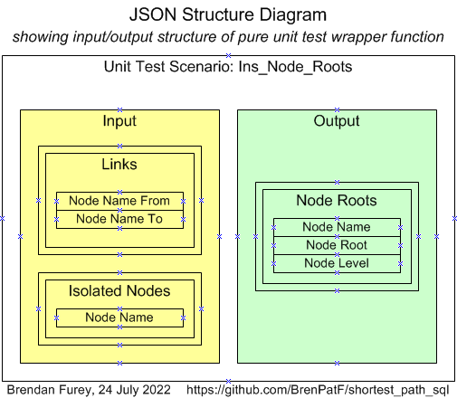
An easy way to generate a starting point for the input JSON file is to use a powershell utility Powershell Utilites module to generate a template file with a single scenario with placeholder records from simple .csv files. See the scripts ins_min_tree_links.ps1, ins_node_roots.ps1 in the unit_test subfolder for an example.
Wrapper Function Code
↑ Unit Test Wrapper Function
↓ Helper Code
↓ Entry Point Functions
This section has the code for the two wrapper functions, starting with the helper code used by both.
Helper Code
The text box below shows the code for the unit test package with private helper units, and placeholder lines for the two wrapper functions, which are included in later text boxes below.
CREATE OR REPLACE PACKAGE BODY TT_Shortest_Path_SQL AS

FUNCTION add_A_Node(
            p_node_name                    VARCHAR2)      -- node name
            RETURN                         PLS_INTEGER IS -- node id
  l_id        PLS_INTEGER;
BEGIN
  SELECT id
    INTO l_id
    FROM nodes
   WHERE node_name = p_node_name;
  RETURN l_id;
EXCEPTION
  WHEN NO_DATA_FOUND THEN
    INSERT INTO nodes (node_name)
    VALUES (p_node_name)
    RETURNING id INTO l_id;
    RETURN l_id;
END add_A_Node;

PROCEDURE add_Nodes(
            p_node_2lis                    L2_chr_arr) IS -- list of node names
  l_id        PLS_INTEGER;
BEGIN
  FOR i IN 1..p_node_2lis.COUNT LOOP
    l_id := add_A_Node(p_node_2lis(i)(1));
  END LOOP;
END add_Nodes;

PROCEDURE add_Links(
            p_link_2lis                    L2_chr_arr) IS -- list of (from node, to node) name pairs
  l_id_fr       PLS_INTEGER;
  l_id_to       PLS_INTEGER;
BEGIN
  EXECUTE IMMEDIATE 'TRUNCATE TABLE links';
  EXECUTE IMMEDIATE 'TRUNCATE TABLE nodes';
  FOR i IN 1..p_link_2lis.COUNT LOOP
    l_id_fr := add_A_Node(p_link_2lis(i)(1));
    l_id_to := add_A_Node(p_link_2lis(i)(2));
    INSERT INTO links VALUES (l_id_fr, l_id_to);
  END LOOP;
END add_Links;

FUNCTION cursor_To_List(
            p_cursor_text                  VARCHAR2)     -- cursor text
            RETURN                         L1_chr_arr IS -- list of delimited records
  l_csr             SYS_REFCURSOR;
BEGIN
  OPEN l_csr FOR p_cursor_text;
  RETURN Utils.Cursor_To_List(x_csr    => l_csr,
                              p_delim  => '|');
END cursor_To_List;

FUNCTION Purely_Wrap_Ins_Min_Tree_Links...
FUNCTION Purely_Wrap_Ins_Node_Roots...

END TT_Shortest_Path_SQL;
Entry Point Functions
Min Pathfinder - Ins_Min_Tree_Links
The text box below shows the code for the unit test wrapper function, Purely_Wrap_Ins_Min_Tree_Links.
FUNCTION Purely_Wrap_Ins_Min_Tree_Links(
            p_inp_3lis                     L3_chr_arr)   -- input list of lists (group, record, field)
            RETURN                         L2_chr_arr IS -- output list of lists (group, record)
  l_act_2lis                     L2_chr_arr := L2_chr_arr();
  l_ins_tot                      PLS_INTEGER;
  l_root_id                      PLS_INTEGER;
BEGIN
  add_Links(p_link_2lis => p_inp_3lis(1));
  add_Nodes(p_node_2lis => p_inp_3lis(2));
  SELECT id
    INTO l_root_id
    FROM nodes
   WHERE node_name = p_inp_3lis(3)(1)(1);
  l_ins_tot := Shortest_Path_SQL.Ins_Min_Tree_Links(l_root_id);
  l_act_2lis.EXTEND(2);
  l_act_2lis(1) := cursor_To_List(p_cursor_text =>
     'SELECT nod.node_name, mtl.lev, nod_p.node_name FROM min_tree_links mtl' ||
     '  JOIN nodes nod ON nod.id = mtl.node_id' ||
     '  LEFT JOIN nodes nod_p ON nod_p.id = mtl.node_id_prior ORDER BY 1');
  ROLLBACK;
  RETURN l_act_2lis;
END Purely_Wrap_Ins_Min_Tree_Links;
Subnetwork Grouper - Ins_Node_Roots
The text box below shows the code for the unit test wrapper function, Purely_Wrap_Ins_Node_Roots.
FUNCTION Purely_Wrap_Ins_Node_Roots(
              p_inp_3lis                     L3_chr_arr)
              RETURN                         L2_chr_arr IS
  l_act_2lis                     L2_chr_arr := L2_chr_arr();
BEGIN
  add_Links(p_link_2lis => p_inp_3lis(1));
  add_Nodes(p_node_2lis => p_inp_3lis(2));
  Shortest_Path_SQL.Ins_Node_Roots(p_node_vsn   => 3,
                                   p_link_vsn   => 5,
                                   p_order_type => 3);
  l_act_2lis.EXTEND;
  l_act_2lis(1) := cursor_To_List(p_cursor_text =>
    'SELECT nod.node_name, rtn.node_name, lev' ||
    '  FROM node_roots nrt' ||
    '  JOIN nodes nod ON nod.id = nrt.node_id' ||
    '  JOIN nodes rtn ON rtn.id = nrt.root_node_id' ||
    ' ORDER BY 2, 1');
  ROLLBACK;
  RETURN l_act_2lis;
END Purely_Wrap_Ins_Node_Roots;
Unit Test Scenarios
↑ Unit Testing
↓ Scenario Category Analysis (SCAN)
↓ Scenario Results
The art of unit testing lies in choosing a set of scenarios that will produce a high degree of confidence in the functioning of the unit under test across the often very large range of possible inputs.
A useful approach to this is to think in terms of categories of inputs, where we reduce large ranges to representative categories. Categories are chosen to explore the full range of potential behaviours of the unit under test. Unit Testing, Scenarios and Categories: The SCAN Method
Scenario Category Analysis (SCAN)
↑ Unit Test Scenarios
↓ Simple Category Sets
↓ Composite Category Sets
↓ Scenario Category Mapping
In this section we identify the category sets for the problem, and tabulate the corresponding categories. We need to consider which category sets can be tested independently of each other, and which need to be considered in combination. We can then obtain a set of scenarios to cover all relevant combinations of categories.
It is helpful first to consider simple category sets, and then go on to consider composite category sets.
In this case we have two entry point APIs to test, and the first of them, Ins_Min_Tree_Links, is called by the second, Ins_Node_Roots. The wrapper function signatures are similar, with both having links and isolated nodes in their inputs and node-based arrays as outputs.
The categories to consider will therefore be very similar, but with an important difference in their application to mapping them to scenarios: Ins_Min_Tree_Links analyses a single subnetwork determined by an input root node, while Ins_Node_Roots analyses the whole network, passing in root nodes to Ins_Min_Tree_Links until all nodes are assigned a subnetwork. The latter can effectively test multiple subnetwork structures in one scenario, wwhile the former will have a scenario for each structure tested.
Simple Category Sets
↑ Scenario Category Analysis (SCAN)
In this section we identify some simple category sets to apply.
SIZ - Size of values By Entity (N-Node only/L-Link)
We want to check that large values, as well as small ones, don’t cause any problems for each entity such as value errors. We can do these in parallel across the entities, and also across other category sets. A node can be isolated and have no link attached, or can be n at least one link, and we want to test both cases.
| Code | Description |
|---|---|
| S | Small values |
| L | Large values |
MBE-X - Multiplicity By Entity (N-Node/L-Link/S-Subnetwork)
We want to check behaviour when there are 0, 1, or more than 1 records for each entity.
| Code | Description |
|---|---|
| 0 | None |
| 1 | One |
| M | Multiple |
NWS-XX - Network Structure
We would like to check the different types of network structure are all handled correctly. We can identify the following types:
- LT - Linear tree
- NT - Nonlinear tree
- LP - Loop :1 and 2-node loops are excluded from datasets, so use 3-node as example
- IL - Isolated link
- IN - Isolated node
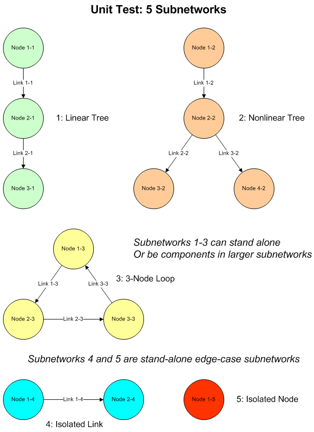
The first three are structures that can be stand-alone subnetworks, or part of a larger subnetwork, while the last two are stand-alone subnetworks by definition. For testing purposes we will use stand-alone subnetworks for all.
For each type the category is Y or N for present or not.
| Code | Description |
|---|---|
| Y | Structure present in network |
| N | Structure not present in network |
Composite Category Sets
↑ Scenario Category Analysis (SCAN)
In this section we consider the Network Structure and Subnetwork Multiplicity category sets in combination, and have one composite category set:
- NWS-XX/MBE-S - Network Structure/Subnetwork Multiplicity
Min Pathfinder - Ins_Min_Tree_Links
While the overall network can contain subnetworks with any or all structures, the Min Pathfinder algorithm starts from a root in a given subnetwork, and the subnetwork will have exactly one of the structures identified. This means we need to test them separately. We will test MBE-S by having the NWS-IL and NWS-IN categories both in a single subnetwork and also as subnetworks in a set of 5 subnetworks.
| NWS-LT | NWS-NT | NWS-LP | NWS-IL | NWS-IN | MBE-S |
|---|---|---|---|---|---|
| Y | N | N | N | N | M |
| N | Y | N | N | N | M |
| N | N | Y | N | N | M |
| N | N | N | Y | N | M |
| N | N | N | N | Y | M |
| N | N | N | Y | N | 1 |
| N | N | N | N | Y | 1 |
The remaining categories can be tested in parallel with these combinations.
Subnetwork Grouper - Ins_Node_Roots
In the case on the Subnetwork Grouper algorithm, we process all subnetworks, making a call to the Min Pathfinder procedure for each, so we can test the different subnetwork structures in one scenario. We will still test MBE-S by having the NWS-IL and NWS-IN categories both in a single subnetwork and also as subnetworks in a set of 5 subnetworks.
| NWS-LT | NWS-NT | NWS-LP | NWS-IL | NWS-IN | MBE-S |
|---|---|---|---|---|---|
| Y | Y | Y | Y | Y | M |
| N | N | N | Y | N | 1 |
| N | N | N | N | Y | 1 |
The remaining categories can be tested in parallel with these combinations.
Scenario Category Mapping
↑ Scenario Category Analysis (SCAN)
We now want to construct a set of scenarios based on the category sets identified, covering each individual category, and also covering combinations of categories that may interact.
Min Pathfinder - Ins_Min_Tree_Links
In this case, the first six category sets listed above may be considered as a single composite set with the combinations listed below forming the scenario keys, while the remaining categories are covered in the first two scenarios.
| # | NWS-LT | NWS-NT | NWS-LP | NWS-IL | NWS-IN | MBE-S | MBE-N | MBE-L | SIZ-N | SIZ-L | Description |
|---|---|---|---|---|---|---|---|---|---|---|---|
| 1 | N | N | N | Y | N | 1 | M | 1 | S | L | Isolated link, large name |
| 2 | N | N | N | N | Y | 1 | 1 | 0 | L | - | Isolated node, large name |
| 3 | Y | N | N | N | N | M | M | M | S | S | 5 subnetworks: trees; isolated link; 3-node loop; isolated node; Root 1-1 |
| 4 | N | Y | N | N | N | M | M | M | S | S | 5 subnetworks: trees; isolated link; 3-node loop; isolated node; Root 1-2 |
| 5 | N | N | Y | N | N | M | M | M | S | S | 5 subnetworks: trees; isolated link; 3-node loop; isolated node; Root 3-3 |
| 6 | N | N | N | Y | N | M | M | M | S | S | 5 subnetworks: trees; isolated link; 3-node loop; isolated node; Root 2-4 |
| 7 | N | N | N | N | Y | M | M | M | S | S | 5 subnetworks: trees; isolated link; 3-node loop; isolated node; Root 1-5 |
Subnetwork Grouper - Ins_Node_Roots
In this case, all network structures can be tested in one scenario, with the remaining categories covered in the first two scenarios.
| # | NWS-LT | NWS-NT | NWS-LP | NWS-IL | NWS-IN | MBE-N | MBE-L | MBE-S | SIZ-N | SIZ-L | Description |
|---|---|---|---|---|---|---|---|---|---|---|---|
| 1 | N | N | N | Y | N | M | 1 | 1 | S | L | Isolated link, large name |
| 2 | N | N | N | N | Y | 1 | 0 | 1 | L | - | Isolated node, large name |
| 3 | Y | Y | Y | Y | Y | M | M | M | S | S | 5 subnetworks: trees; isolated link; 3-node loop; isolated node |
Scenario Results
↑ Unit Test Scenarios
↓ Results Summary
↓ Unit Test Report: Oracle SQL Shortest Paths: Node Tree
↓ Unit Test Report: Oracle SQL Shortest Paths: Node Roots
Results Summary
Unit Test Results Summary for Folder ./externals/shortest_path_sql
==================================================================
 File                                                          Title                                  Inp Groups  Out Groups  Tests  Fails  Folder
-------------------------------------------------------------  -------------------------------------  ----------  ----------  -----  -----  -------------------------------------
 tt_shortest_path_sql.purely_wrap_ins_min_tree_links_out.json  Oracle SQL Shortest Paths: Node Tree            3           2      7      0  oracle-sql-shortest-paths_-node-tree
 tt_shortest_path_sql.purely_wrap_ins_node_roots_out.json      Oracle SQL Shortest Paths: Node Roots           2           2      3      0  oracle-sql-shortest-paths_-node-roots

0 externals failed, see ./externals/shortest_path_sql for scenario listings
The formatted results files, both text and HTML, are available in the GitHub project unit_test/output subfolders. The summary reports showing scenarios tested, plus an example scenario report, in text format, are shown below.
Unit Test Report: Oracle SQL Shortest Paths: Node Tree
Unit Test Report: Oracle SQL Shortest Paths: Node Tree
Here is the root page for the Node Tree unit test results in text format:
Unit Test Report: Oracle SQL Shortest Paths: Node Tree
======================================================

      #    Scenario                                                                   Fails (of 2)  Status
      ---  -------------------------------------------------------------------------  ------------  -------
      1    Isolated link, large name                                                  0             SUCCESS
      2    Isolated node, large name                                                  0             SUCCESS
      3    5 subnetworks: trees; isolated link; 3-node loop; isolated node; Root 1-1  0             SUCCESS
      4    5 subnetworks: trees; isolated link; 3-node loop; isolated node; Root 1-2  0             SUCCESS
      5    5 subnetworks: trees; isolated link; 3-node loop; isolated node; Root 3-3  0             SUCCESS
      6    5 subnetworks: trees; isolated link; 3-node loop; isolated node; Root 2-4  0             SUCCESS
      7    5 subnetworks: trees; isolated link; 3-node loop; isolated node; Root 1-5  0             SUCCESS

Test scenarios: 0 failed of 7: SUCCESS
======================================
Scenarioo 3: 5 subnetworks: trees; isolated link; 3-node loop; isolated node; Root 1-1
Here, as an example, is the scenario 3 page for the Node Tree unit test results in text format:
SCENARIO 3: 5 subnetworks: trees; isolated link; 3-node loop; isolated node; Root 1-1 {
=======================================================================================
   INPUTS
   ======
      GROUP 1: Input Links {
      ======================
            #  Node Name From  Node Name To
            -  --------------  ------------
            1  Node 1-1        Node 2-1
            2  Node 2-1        Node 3-1
            3  Node 1-2        Node 2-2
            4  Node 2-2        Node 3-2
            5  Node 2-2        Node 4-2
            6  Node 1-3        Node 2-3
            7  Node 2-3        Node 3-3
            8  Node 3-3        Node 1-3
            9  Node 1-4        Node 2-4
      }
      =
      GROUP 2: Isolated Nodes {
      =========================
            #  Node Name
            -  ---------
            1  Node 1-5
      }
      =
      GROUP 3: Root {
      ===============
            #  Node Name
            -  ---------
            1  Node 1-1
      }
      =
   OUTPUTS
   =======
      GROUP 1: Node Tree {
      ====================
            #  Node Name  Node Level  Prior Node
            -  ---------  ----------  ----------
            1  Node 1-1   0
            2  Node 2-1   1           Node 1-1
            3  Node 3-1   2           Node 2-1
      } 0 failed of 3: SUCCESS
      ========================
      GROUP 2: Unhandled Exception: Empty as expected: SUCCESS
      ========================================================

} 0 failed of 2: SUCCESS
========================
You can review the HTML formatted unit test results here:
Unit Test Report: Oracle SQL Shortest Paths: Node Roots
Unit Test Report: Oracle SQL Shortest Paths: Node Roots
Here is the root page for the Node Roots unit test results in text format:
Unit Test Report: Oracle SQL Shortest Paths: Node Roots
=======================================================

      #    Scenario                                                         Fails (of 2)  Status
      ---  ---------------------------------------------------------------  ------------  -------
      1    Isolated link, large name                                        0             SUCCESS
      2    Isolated node, large name                                        0             SUCCESS
      3    5 subnetworks: trees; isolated link; 3-node loop; isolated node  0             SUCCESS

Test scenarios: 0 failed of 3: SUCCESS
======================================
You can review the HTML formatted unit test results here:
Conclusion
We have shown how network path problems can be solved using SQL queries alone, but that for larger, looped networks the queries become impractical.
Two more scalable algorithms have been proposed for finding shortest paths, and for subnetwork grouping, and have been first explained in abstract terms. They have then been implemented in PL/SQL with embedded SQL and tables to store intermediate solutions.
We have applied these PL/SQL programs to a range of datasets, upto a size of 2,800,309 nodes and 109,262,592 links, and obtained solutions for all of them.
We have applied several methods for execution time profiling, including the author’s own code timing package Timer_Set, and identified tuning opportunities for the subnetwork grouping procedure.
These tuning opportunities involved, in one case, treating simple subnetworks separately, to be inserted by single SQL statements ahead of the main algorithm. This led to exploration of the performance of several alternative SQL implementations using Oracle’s Execution Plan instrumentation.
In the second case, alternatives were explored for the most intensive line in the base version, which selected a new root node for each succeeding subnetwork. These optimizations resulted in a 5-7-fold improvement in performance on the largest datasets.
Finally, we showed how the programs can be tested using the Math Function Unit Testing design pattern, Trapit - Oracle PL/SQL unit testing module.
References
- SQL and PL/SQL for Shortest Path Problems: GitHub, Brendan Furey, August 2022
- SQL for Shortest Path Problems, Brendan Furey, April 2015
- SQL for Shortest Path Problems 2: A Branch and Bound Approach, Brendan Furey, May 2015
- PL/SQL Pipelined Function for Network Analysis, Brendan Furey, May 2015
- PL/SQL Profiling 1: Overview, Brendan Furey, June 2020
- Friendship network of Brightkite users, Jure Leskovec, Stanford University, Undated
- Bacon Numbers Datasets from Oberlin College, December 2016
- Using the PostgreSQL Recursive CTE - Part Two, Bryn Llewellyn, March 2021
- Unit Testing, Scenarios and Categories: The SCAN Method, Brendan Furey, October 2021
- Trapit - Oracle PL/SQL unit testing module: GitHub, Brendan Furey, June 2016
- Timer_Set - Oracle PL/SQL code timing module: GitHub, Brendan Furey, January 2019
- Powershell utilities module: GitHub, Brendan Furey, August 2019