Coupons, Caps and Functions
On 18 April 2025 a poster asked a question on the AskTom Oracle forum: Solving a logical problem using analytical functions. The problem turned out to be surprisingly difficult to solve in pure SQL.
I posted two solution methods on the thread for a generalised form of the problem. One solution used Oracle’s MODEL clause, the other a pipelined function. In this article, I explain how these work, and add a third method based on recursive subquery factoring. In addition, I analyse the performance characteristics of the three methods using an approach I presented at the 2017 Irish Oracle User Group conference in Dublin, Dimensional Performance Benchmarking of SQL. The analysis includes curve-fitting using Excel graphs and statistical functions.
The methods are tested using The Math Function Unit Testing Design Pattern, with test results in HTML and text format included.
Everything is automated.
GitHub 
Contents
↓ The Coupons and Caps Allocation Problem
↓ Functions, Fonctions, Funktionen
↓ Solutions Code
↓ Performance Testing
↓ Unit Testing
↓ Conclusion
↓ See Also
The Coupons and Caps Allocation Problem
↑ Contents
↓ Problem Definition
↓ Data Model
↓ Worked Example
In this section, we define the problem to be solved, starting from the original poster’s definition on the AskTom Oracle forum.
Problem Definition
↑ The Coupons and Caps Allocation Problem
The poster, ST, defines the problem in this way ( Solving a logical problem using analytical functions):
I am trying to solve a problem using analytical functions but I am stuck.
- I have a list of coupons that I can use. The usage sequence is in alphabetical order of the coupon name.
- There is a limit (cap) on the total value across all coupons that can be used in a day
- Each coupon is subject to 1 or 2 caps. If it is subject to 2 caps, there is a specified sequence to apply caps.
- I have to now find how much coupon value could be utilized before my daily cap was reached. i.e. find “coupon usage” and “Cap Remaining” below.
I am able to make this work using analytical function with a single cap. The 2 caps with a possibly different usage sequence has me stuck.
We will develop methods to solve the more general problem where there can be any number of caps, but we’ll start by reviewing the example problem provided by the poster.
Data Model
↑ The Coupons and Caps Allocation Problem
↓ ERD
↓ DDL
↓ Example Data
ERD

DDL
CREATE TABLE coupon_data (
	coupon 			VARCHAR2(10),
	value 			INTEGER,
	CONSTRAINT cou_pk PRIMARY KEY (coupon))
/
PROMPT Create cap_data
CREATE TABLE cap_data (
	cap_name 		VARCHAR2(10),
	cap_limit 		INTEGER,
	CONSTRAINT cap_pk PRIMARY KEY (cap_name))
/
CREATE TABLE coupon_cap_mapping (
	coupon 			VARCHAR2(10),
	cap_name 		VARCHAR2(10),
	cap_sequence  	INTEGER,
	CONSTRAINT ccm_pk PRIMARY KEY (coupon, cap_sequence))
/
Example Data
↑ Data Model
The following SQL creates the data corresponding to the poster’s example.
INSERT INTO coupon_data
WITH data ( coupon, value ) AS (
	SELECT 'A', 100 FROM DUAL UNION ALL
	SELECT 'B', 40  FROM DUAL UNION ALL
	SELECT 'C', 120 FROM DUAL UNION ALL
	SELECT 'D', 10  FROM DUAL UNION ALL
	SELECT 'E', 200 FROM DUAL
)
SELECT * FROM data
/
INSERT INTO cap_data
WITH data  ( cap_name, cap_limit ) AS (
	SELECT 'Cap 1', 150 FROM DUAL UNION ALL
	SELECT 'Cap 2', 70  FROM DUAL
)
SELECT * FROM data
/
INSERT INTO coupon_cap_mapping
WITH data  ( coupon, cap_name, cap_sequence ) AS (
	SELECT 'A', 'Cap 1', 1 FROM DUAL UNION ALL
	SELECT 'A', 'Cap 2', 2 FROM DUAL UNION ALL
	SELECT 'B', 'Cap 2', 1 FROM DUAL UNION ALL
	SELECT 'C', 'Cap 2', 1 FROM DUAL UNION ALL
	SELECT 'C', 'Cap 1', 2 FROM DUAL UNION ALL
	SELECT 'D', 'Cap 1', 1 FROM DUAL UNION ALL
	SELECT 'E', 'Cap 1', 1 FROM DUAL UNION ALL
	SELECT 'E', 'Cap 2', 2 FROM DUAL
)
SELECT * FROM data
/
Worked Example
↑ The Coupons and Caps Allocation Problem

The diagram illustrates the example problem provided by the original poster on the AskTom thread, with 5 coupons, 2 caps, and the mapping and values supplied. The columns on the right show how the solution can be found in a sequence of 8 iterations. The columns are:
- Coupon Usage: Usage of coupon on a single cap at a given iteration
- Coupon Left: Amount of coupon left after its usage at a given iteration
- Cap 1 Left: Amount of cap 1 left after the usage at a given iteration
- Cap 2 Left: Amount of cap 2 left after the usage at a given iteration
The coupon values at each iteration depend on the initial coupon value for each new coupon, then on the amount left for subsequent iterations.
The cap values depend first on the initial cap values, then at each subsequent iteration, on the values left at the previous iteration.
The x/y bubbles connected by arrows show how the iteration scheme proceeds in coupon order, completing processing of each coupon before moving to the next.
The solution process presented here seems straightforward enough. However, implementing it in pure SQL is not so easy, especially if we want to allow an arbitrary number of caps. In fact, it’s not possible to do this using analytic functions alone, as the original poster thought: Some form of recursion is required in order to keep track of the values left.
We’ll show how to solve the more general problem in three different ways:
- Pipelined function: This solution uses PL/SQL with an associative array to track the cap left values
- MODEL clause: This solution uses an iterative MODEL clause with cap left values tracked by array position
- Recursive subquery factoring: This solution uses a recursive query where each iteration corresponds to a single coupon with rows for each cap
The queries will turn out to have quite different performance characteristics.
Functions, Fonctions, Funktionen
[Login to Spotify on your browser to allow for full Kraftwerk accompaniments 🎧]
All programmers are familiar with the idea of a function as a unit of code that takes input parameters, performs some sequence of steps, and then returns a value. However, the concept of a function in a more abstract sense has a much wider applicability within IT. Functional Programming, in particular, emphasises the benefits of designing programs around pure functions, which return values deterministically and without side effects.
We highlight here three distinct ways in which the concept of the function is applied in the current article:
- The Math Function Unit Testing Design Pattern
- The solution queries described here are tested using this design pattern, which I developed around the idea that an externally pure wrapper function enables fully automated, repeatable, unit testing
- Dimensional Performance Benchmarking of SQL
- In 2017 I presented on this subject at the Irish Oracle User Group conference in Dublin. The approach, which is used in the current article, evaluates the performance characteristics of alternative solution methods by regarding execution time as a function of parameters defining dataset size
- Curve-Fitting
- This technique models a set of observed (x, y) values as approximating an underlying function, such as a polynomial or a power-law function, with unknown coefficients. The size of the discrepancies between the observed y-values and the function’s predictions can be viewed as another function, with the coefficients as x-values, and optimal coefficients can be obtained by minimizing the value of this derived function
Solutions Code
↑ Contents
↓ Pipelined Function (PLF)
↓ The MODEL Clause (MOD)
↓ Recursive Subquery Factoring (RSF)
↓ Views
There are two solution methods in pure SQL and one that consists of a PL/SQL pipelined function with embedded SQL and associated object types.
Pipelined Function (PLF)
↑ Solutions Code
↓ Object Type Definitions
↓ Function Definition
↓ Notes on PLF
↓ View
Object Type Definitions
CREATE OR REPLACE TYPE caps_obj AS OBJECT (
        coupon          VARCHAR2(10),
        value           INTEGER,
        cap_name        VARCHAR2(10),
        cap_sequence    INTEGER,
        cap_limit       INTEGER,
        usage           INTEGER,
        val_left        INTEGER,
        cap_left        INTEGER
)
/
CREATE OR REPLACE TYPE caps_tab AS TABLE OF caps_obj
/
Function Definition
CREATE OR REPLACE FUNCTION caps RETURN caps_tab PIPELINED IS
    CURSOR cap_coupon_csr IS
    SELECT cou.coupon,
           cou.value,
           cap.cap_name,
           ccm.cap_sequence,
           cap.cap_limit
      FROM cap_data           cap
      JOIN coupon_cap_mapping ccm ON ccm.cap_name = cap.cap_name
      JOIN coupon_data        cou ON cou.coupon = ccm.coupon
     ORDER BY cou.coupon, ccm.cap_sequence;
    l_pri_coupon            VARCHAR2(10) := 'NA';
    TYPE cap_left_ibt IS    TABLE OF NUMBER INDEX BY VARCHAR2(10);
    l_cap_left              cap_left_ibt;
    l_usage                 PLS_INTEGER;
    l_val_left              PLS_INTEGER;
BEGIN
    FOR rec IN (SELECT cap_name, cap_limit FROM cap_data) LOOP
        l_cap_left(rec.cap_name) := rec.cap_limit;
    END LOOP;
    FOR rec IN cap_coupon_csr LOOP
        IF rec.coupon != l_pri_coupon THEN
            l_val_left := rec.value;
        END IF;
        l_usage                  := Least (l_val_left, l_cap_left(rec.cap_name));
        l_val_left               := l_val_left - l_usage;
        l_cap_left(rec.cap_name) := l_cap_left(rec.cap_name) - l_usage;
        l_pri_coupon             := rec.coupon;
        PIPE ROW(caps_obj(rec.coupon,
                          rec.value,
                          rec.cap_name,
                          rec.cap_sequence,
                          rec.cap_limit,
                          l_usage,
                          l_val_left,
                          l_cap_left(rec.cap_name)));
    END LOOP;
END caps;
/
Notes on PLF
This is a very simple implementation of the algorithm outlined in the worked example, allowing for arbitrary numbers of caps.
- The cursor cap_coupon_csr simply inner-joins the three tables, ordering by coupon and cap_sequence
- The cap left values are tracked using an associative array, indexed by cap name, and initialized with the cap limits
- The coupon amount left is initialized with coupon value within the loop whenever the coupon changes
- Usage is then the lower of the coupon amount left and the cap left for current coupon and cap
- The left values are then updated accordingly, and the row is piped out
View
CREATE OR REPLACE VIEW coupon_caps_plf_v AS
SELECT * FROM TABLE(caps)
/
The MODEL Clause (MOD)
↑ Solutions Code
↓ Notes on MOD
CREATE OR REPLACE VIEW coupon_caps_mod_v AS
WITH cap_coupon_map AS (
SELECT Row_Number() OVER (ORDER BY cou.coupon, ccm.cap_sequence) ccm_ind,
       cou.coupon,
       cou.value,
       cap.cap_name,
       ccm.cap_sequence,
       cap.cap_limit
  FROM cap_data           cap
  JOIN coupon_cap_mapping ccm ON ccm.cap_name = cap.cap_name
  JOIN coupon_data        cou ON cou.coupon = ccm.coupon
)
SELECT *
  FROM cap_coupon_map
MODEL
  DIMENSION BY (ccm_ind)
  MEASURES (Lag(ccm_ind, 1, ccm_ind) OVER (PARTITION BY cap_name ORDER BY coupon) pri_ccm_ind,
            coupon,
            Lag(coupon, 1, 'NA') OVER (ORDER BY ccm_ind) pri_coupon,
            value,
            cap_name,
            cap_sequence,
            cap_limit,
            0 usage,
            value val_left,
            cap_limit cap_left)
  RULES UPDATE ITERATE (1000000) UNTIL coupon[ITERATION_NUMBER + 1] IS NULL (
    usage[ITERATION_NUMBER + 1]     = CASE WHEN coupon[ITERATION_NUMBER + 1] != pri_coupon[ITERATION_NUMBER + 1] THEN
                                                    Least (val_left[ITERATION_NUMBER + 1], cap_left[pri_ccm_ind[ITERATION_NUMBER + 1]])
                                           ELSE     Least (val_left[ITERATION_NUMBER], cap_left[pri_ccm_ind[ITERATION_NUMBER + 1]])
                                      END,
    val_left[ITERATION_NUMBER + 1]  = CASE WHEN coupon[ITERATION_NUMBER + 1] != pri_coupon[ITERATION_NUMBER + 1] THEN
                                                    val_left[ITERATION_NUMBER + 1] - usage[ITERATION_NUMBER + 1]
                                           ELSE     val_left[ITERATION_NUMBER] - usage[ITERATION_NUMBER + 1]
                                      END,
    cap_left[ITERATION_NUMBER + 1]  = cap_left[pri_ccm_ind[ITERATION_NUMBER + 1]] - usage[ITERATION_NUMBER + 1]
  )
/
Notes on MOD
The iterative form of MODEL clause, with sequential ordering, is needed here where a given row depends on values in prior rows.
- The subquery cap_coupon_map inner-joins the three tables, and adds an index column representing the ordering by coupon and cap_sequence to be used as the MODEL dimension
- The measure pri_ccm_ind is the prior index for the current cap, defaulting to current index
- The measure pri_coupon is the prior coupon in the row set, defaulting to ‘NA’
- Each iteration corresponds to a row in the subquery rowset in order of the index column
- Usage is calculated with similar logic to the PLF method, but with current cap left being referenced from the cap left value of the prior cap row, via the pri_ccm_ind measure
- The new left values are then again calculated accordingly
- ITERATION_NUMBER starts at zero, but the dimension starts at 1
- Termination occurs when the new coupon is null, meaning the last row has been processed
Recursive Subquery Factoring (RSF)
↑ Solutions Code
↓ Notes on RSF
CREATE OR REPLACE VIEW coupon_caps_rsf_v AS
WITH coupons AS (
    SELECT cou.coupon,
           Row_Number() OVER (ORDER BY cou.coupon) cou_ind,
           cou.value
      FROM coupon_data cou
     WHERE EXISTS (SELECT 1 FROM coupon_cap_mapping ccm WHERE ccm.coupon = cou.coupon)
), rsf (coupon, cou_ind, value, cap_name, cap_sequence, cap_limit, usage, cap_left) AS (
    SELECT NULL coupon,
           0 cou_ind,
           0 value,
           cap_name,
           0 cap_sequence,
           cap_limit,
           0 usage,
           cap_limit cap_left
      FROM cap_data
     UNION ALL
    SELECT cou.coupon,
           cou.cou_ind,
           cou.value,
           cap.cap_name,
           ccm.cap_sequence,
           rsf.cap_limit,
           Greatest(0, Least(cou.value -
                Nvl(Sum(rsf.cap_left)
                    OVER (ORDER BY ccm.cap_sequence
                          ROWS BETWEEN UNBOUNDED PRECEDING AND 1 PRECEDING), 0), rsf.cap_left)) usage,
           rsf.cap_left -
           Nvl2(ccm.cap_sequence, Greatest(0, Least(cou.value -
                Nvl(Sum(rsf.cap_left)
                    OVER (ORDER BY ccm.cap_sequence
                          ROWS BETWEEN UNBOUNDED PRECEDING AND 1 PRECEDING), 0), rsf.cap_left)), 0) cap_left
      FROM rsf
      JOIN coupons cou ON cou.cou_ind = rsf.cou_ind + 1
      JOIN cap_data cap ON cap.cap_name = rsf.cap_name
      LEFT JOIN coupon_cap_mapping ccm ON ccm.coupon = cou.coupon AND ccm.cap_name = rsf.cap_name
)
SELECT coupon, cou_ind, value, cap_name, cap_sequence, cap_limit, usage,
        value - Sum(usage) OVER (PARTITION BY coupon ORDER BY cap_sequence) val_left,
        cap_left
  FROM rsf
 WHERE coupon IS NOT NULL AND cap_sequence IS NOT NULL
/
Notes on RSF
↑ Recursive Subquery Factoring (RSF)
Each iteration of the recursive query corresponds to the processing of a single coupon, and can only see the rowset from the prior iteration. This means that, in order to track the cap left values, they must be passed through each iteration. Therefore the anchor branch selects all records from CAP_DATA, and the recursive branch outer-joins COUPON_CAP_MAPPING, with null value for cap_sequence meaning absence of a mapping between coupon and cap.
The expressions for usage and cap_left are built up in stages:
- The inner analytic Sum(rsf.cap_left) gets the running sum of cap_left for the coupon from the first upto the cap prior to the current cap, based on the cap_sequence ordering for the coupon
- This value will be null at the first cap for the coupon, so take that as zero using Nvl
- Subtracting this from the coupon value gives the amount of coupon left for the current cap
- The lower of this value and the current cap_left is the provisional usage, but could be negative, in which case the usage is zero
- Note that the cap_sequence for the current row could be null, meaning usage should be zero: This is taken into account in the next expression, and the null cap_sequence rows are excluded in the final Where condition, so this does not cause an error
- The provisional cap_left is the previous cap_left minus the usage expression, but only if the cap_sequence is not null, else cap_left is unchanged
The expression for val_left uses an analytic running sum partitioned by coupon in the main section.
Views
↑ Solutions Code
↓ Views for Unit Testing
↓ Views for Performance Testing
Views for Unit Testing
The queries have been created as views, which is convenient for unit testing, as described in the preceding sections. Each view, COUPON_CAPS_xxx_V, for xxx in (PLF, MOD, RSF) with an additional version having a bug, COUPON_CAPS_RSF_BUG_V, of the correct COUPON_CAPS_RSF_V, has the following columns:
- coupon
- cou_ind
- value
- cap_name
- cap_sequence
- cap_limit
- usage
- val_left
- cap_left
Views for Performance Testing
It is convenient for performance testing to create additional aggregation views that return a single row. Each aggregation view, COUPON_CAPS_xxx_AGG_V, for xxx in (PLF, MOD, RSF) has the form:
COUPON_CAPS_xxx_AGG_V
CREATE OR REPLACE VIEW coupon_caps_xxx_agg_v AS
SELECT Count(CASE WHEN usage > 0 THEN 1 END) n_pos_usages,
       Count(*) n_rows,
       Sum(usage) sum_usage
  FROM coupon_caps_xxx_v
/
The columns are:
- n_pos_usages: number of rows with positive usage
- n_rows: total number of rows
- sum_usage: sum of usages
These views also help to verify that, at each data point, the different queries return the same result set.
Performance Testing
↑ Contents
↓ Dimensional Benchmarking
↓ Curve Fitting Using Polynomial and Power-Law Functions
↓ Test Data
↓ Running the Performance Testing
↓ Results
Dimensional Benchmarking
In 2017 I presented Dimensional Performance Benchmarking of SQL at the Irish Oracle User Group conference in Dublin. In the presentation it’s explained how, using generated datasets with parameters that control the dataset size in multiple dimensions, it’s possible to explore performance variation across the dimensions. This approach can provide much richer information on the performance characteristics of a computational algorithm, including SQL queries in particular, than just running on a few datasets.
We’ll follow this approach here, where the following dataset parameters suggest themselves:
- number of coupons (#Cou)
- number of caps assigned to a coupon (#Cap/Cou)
- number of caps (#Cap)
We can assign minimum and maximum values for the coupons and caps, and create randomized values within these limits according to the parameters. For simplicity, we will use single values for the #Cap/Cou parameter across all coupons, and assign the #Cap/Cou caps randomly to each coupon.
In this case we choose 6 values for each of the parameters, then run performance tests on the solution methods across the range of each parameter, while holding the other two parameters fixed at their maximum sizes. We will capture the elapsed times for each method at each data point, and it will be convenient to use my Oracle PL/SQL Code Timing Module, which allows the results to be read in a simple tabular format.
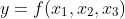
We can express what we are doing symbolically, using y to represent the dependent variable, elapsed time, and  the parameters as independent variables, with f being the (unknown) underlying function:
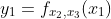
Then, if we use subscripts to represent the fixed parameter variables, we have three functions of a single independent variable, thus:
Curve Fitting Using Polynomial and Power-Law Functions
↑ Performance Testing
↓ Least Squares for Polynomial Curve-Fitting
↓ Least Squares for Power-Law Curve-Fitting
↓ Coefficient of Determination
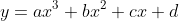
Curve-fitting techniques are extremely useful in trying to understand the variation in elapsed time with parameter variation. We’ll consider both polynomial curves, upto order 3, like this:
and power-law curves like this:

Least Squares for Polynomial Curve-Fitting
↑ Curve Fitting Using Polynomial and Power-Law Functions
First, consider the case of the third order polynomial. If we have a set of n data points, using i = 1,…,n as an index, and  the i’th data point, we can define the residual error at data point i for a set of coefficients (a, b, c, d) as:

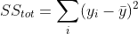
This allows us to define a measure of the total errors as the sum of the squares of the residuals,  , thus:

It is possible to find the minimum of this function by equating the four partial derivatives with respect to the variables to zero, which results in a set of linear equations. We don’t need to go into the details here, but read this Wikipedia article for more information, Least squares, including some of the history of the method, such as:
The first clear and concise exposition of the method of least squares was published by Legendre in 1805.
Excel Formulas for Coefficients
The coefficients minimizing the error function can be obtained using an Excel function.
Cubic Polynomial
The following expression returns the cubic least squares coefficients a, b, c and d in the four adjacent cells starting with the formula cell:
=LINEST(B4:B9, A4:A9^{1,2,3}, TRUE, FALSE)
This assumes the y-values are in the range B4:B9 and the x-values in the range A4:A9
Straight Line
The following expression returns the linear least squares coefficients a and b in the two adjacent cells starting with the formula cell:
=LINEST(B4:B9,A4:A9)
Least Squares for Power-Law Curve-Fitting
↑ Curve Fitting Using Polynomial and Power-Law Functions
We can apply the same least squares method to fitting a power-law curve:
by taking logs:
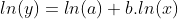
Replacing the x and y values by logarithms, we have a linear equation and can apply the method to solve for b and ln(a).
Excel Formulas for Coefficients
The following expression returns the linear least squares coefficients b and ln(a) in the two adjacent cells starting with the formula cell:
=LINEST(LN(B4:B9),LN(A4:A9))
We then obtain a as:
=EXP(B24)
assuming ln(a) is in cell B24.
Coefficient of Determination
↑ Curve Fitting Using Polynomial and Power-Law Functions
This section is based on the Wikipedia article, Coefficient of determination, from which the following definition is taken:
In statistics, the coefficient of determination, denotedand pronounced "R squared", is the proportion of the variation in the dependent variable that is predictable from the independent variable(s).
With , the sum of squares of residuals, defined as above,  the mean of the y-values, and
  , the sum of squares of differences from the mean (proportional to the variance) defined thus:
the coefficient of determination, , is defined thus:
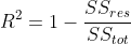
A larger value of
Excel Formula for Coefficient of Determination
The following expression returns the coefficient of determination, assuming the observed y-values are in the range B4:B9 and the predicted y-values in the range C4:C9:
=1 - (SUMXMY2($B4:$B9, C4:C9) / DEVSQ($B4:$B9))
Test Data
↑ Performance Testing
↓ Datasets
↓ Create Test Data
As discussed in the Dimensional Benchmarking section above we want to create randomized test datasets parametrized by three variables.
Datasets
For the PLF and MOD queries only, we used the following parameter ranges:
- #Cou: (10000, 20000, 30000, 40000, 50000, 60000)
- #Cap/Cou: (2, 4, 6, 8, 10, 12)
- #Cap: (12, 14, 16, 18, 20, 22)
The RSF query turned out to be much longer-running than the other two and needed a smaller set of #Cou values to run in reasonable times, so we used values ten times smaller:
- #Cou: (1000, 2000, 3000, 4000, 5000, 6000)
All three queries were run on this smaller set of datasets, to verify that result sets were the same, but only the RSF timings were analysed in detail.

Create Test Data
The following procedure, in the package Coupon_Caps, deletes existing data and inserts a new randomized dataset, with numbers of records determined by the input parameters.
PROCEDURE Create_Test_Data(
            p_n_cou                        PLS_INTEGER,
            p_n_cap                        PLS_INTEGER,
            p_n_cap_per_cou                PLS_INTEGER) IS
  l_int       PLS_INTEGER;
  l_count     PLS_INTEGER;
  l_cou       VARCHAR2(10);
  l_cap       VARCHAR2(10);

  FUNCTION Rand_Int (
              p_min                          PLS_INTEGER,
              p_max                          PLS_INTEGER)
              RETURN                         PLS_INTEGER IS
  BEGIN
    RETURN TRUNC(DBMS_RANDOM.VALUE(p_min, p_max + 1));
  END Rand_Int;

BEGIN
  DELETE coupon_cap_mapping;
  DELETE cap_data;
  DELETE coupon_data;
  FOR i IN 1..p_n_cou LOOP
    l_int := Rand_Int(MIN_COU, MAX_COU);
    l_cou := 'COU' || LPad(i - 1, 5, '0');
    INSERT INTO coupon_data ( coupon, value )
    VALUES (l_cou, l_int);
    FOR j IN 1..p_n_cap_per_cou LOOP
      l_count := 0;
      WHILE l_count = 0 LOOP
        l_int := Rand_Int(1, p_n_cap);
        l_cap := 'CAP' || LPad(l_int - 1, 2, '0');
        INSERT INTO coupon_cap_mapping
        SELECT l_cou, l_cap, j
          FROM DUAL
         WHERE NOT EXISTS (SELECT 1 FROM coupon_cap_mapping ccm
                            WHERE ccm.coupon = l_cou
                              AND ccm.cap_name = l_cap);
        l_count := SQL%ROWCOUNT;
      END LOOP;
    END LOOP;
  END LOOP;
  FOR i IN 1..p_n_cap LOOP
    l_int := Rand_Int(MIN_CAP, MAX_CAP);
    INSERT INTO cap_data VALUES ('CAP' || LPad(i - 1, 2, '0'), l_int);
  END LOOP;
  DBMS_Stats.Gather_Schema_Stats(ownname => 'APP');
  Utils.L('create_Test_Data ' || p_n_cou || ' - ' || p_n_cap_per_cou || ' - ' || p_n_cap);
END Create_Test_Data;
Running the Performance Testing
↑ Performance Testing
↓ Oracle Script to Run Views on a Data Point
↓ Oracle Procedure Run_Data_Point
↓ Performance Testing PowerShell Script
[Schema: app; Folder: performance_testing; Script: Run-All.ps1]
The running of the queries on all datasets is completely automated, using a PowerShell script, Run-All.ps1, that calls a sqlplus script, run_dp.sql, at each data point.
Oracle Script to Run Views on a Data Point
↑ Running the Performance Testing
This sqlplus script is passed dataset parameters from the driving PowerShell script, and calls the Run_Data_Point procedure to run and time the views, using the TIMER_SET bind variable.
run_dp.sql
DEFINE N_COU = &1
DEFINE N_CAP_PER_COU = &2
DEFINE N_CAP = &3
DEFINE N_VIEWS = &4
DEFINE XPLAN_YN = '&5'
PROMPT Create data - &N_COU coupons, &N_CAP_PER_COU caps per coupon, &N_CAP caps
TRUNCATE TABLE coupon_cap_mapping
/
TRUNCATE TABLE cap_data
/
TRUNCATE TABLE coupon_data
/
DECLARE
  l_n_cou               PLS_INTEGER := &N_COU;
  l_n_cap_per_cou       PLS_INTEGER := &N_CAP_PER_COU;
  l_n_cap               PLS_INTEGER := &N_CAP;
  l_n_views             PLS_INTEGER := &N_VIEWS;
  l_get_xplan           BOOLEAN := '&XPLAN_YN' = 'Y';
BEGIN
  Coupon_Caps.Run_Data_Point(
            p_n_cou           => l_n_cou,
            p_n_cap_per_cou   => l_n_cap_per_cou,
            p_n_cap           => l_n_cap,
            p_n_views         => l_n_views,
            p_ts              => :TIMER_SET,
            p_get_xplan       => l_get_xplan);
END;
/
Oracle Procedure Run_Data_Point
↑ Running the Performance Testing
The following procedure first calls Create_Test_Data to set up the dataset at a given point, then runs and times each view (excluding RSF if p_n_views = 2), with conditional logic around detail of timing, and whether to get an execution plan.
Coupon_Caps.Run_Data_Point
PROCEDURE Run_Data_Point(
            p_n_cou                        PLS_INTEGER,
            p_n_cap_per_cou                PLS_INTEGER,
            p_n_cap                        PLS_INTEGER,
            p_n_views                      PLS_INTEGER,
            p_ts                           PLS_INTEGER,
            p_get_xplan                    BOOLEAN := FALSE) IS
  l_view_lis            L1_chr_arr := L1_chr_arr('coupon_caps_plf_agg_v', 'coupon_caps_mod_agg_v', 'coupon_caps_rsf_agg_v');
  l_dp_name             VARCHAR2(100) := p_n_cou || ' - ' || p_n_cap_per_cou || ' - ' || p_n_cap;
  PROCEDURE do_Run (
            p_view_name                    VARCHAR2,
            p_get_xplan                    BOOLEAN,
            p_timer_detail                 BOOLEAN) IS
    l_act_lis             L1_chr_arr;
    l_timer_name          VARCHAR2(100) := 'Sum-' || p_view_name;
    l_timer_name_det      VARCHAR2(100) := p_view_name || ' ' || l_dp_name;
    l_search              VARCHAR2(100) := p_view_name || TRUNC(DBMS_RANDOM.VALUE(100000, 999999));
  BEGIN
    IF p_get_xplan THEN
      l_timer_name := 'XPLAN-' || l_timer_name;
      l_timer_name_det := 'XPLAN-' || l_timer_name_det;
    END IF;
    IF p_timer_detail THEN
      l_timer_name := l_timer_name_det;
    END IF;
    l_act_lis := Utils.View_To_List(
                                p_view_name     => p_view_name,
                                p_sel_value_lis => L1_chr_arr('n_pos_usages', 'n_rows', 'sum_usage'),
                                p_hint          => CASE WHEN p_get_xplan THEN 'gather_plan_statistics ' || l_search END);
    Timer_Set.Increment_Time(p_ts, l_timer_name);
    IF p_get_xplan THEN
      Utils.L(Utils.Get_XPlan(p_sql_marker => l_search));
    END IF;
    Utils.L('Result for ' || l_timer_name_det || ': ' || l_act_lis(1));
  END do_Run;
BEGIN
  Create_Test_Data(
            p_n_cou           => p_n_cou,
            p_n_cap           => p_n_cap,
            p_n_cap_per_cou   => p_n_cap_per_cou);
  Timer_Set.Increment_Time(p_ts, 'create_Test_Data: ' || l_dp_name);
  FOR i IN 1..p_n_views LOOP
    do_Run(p_view_name    => l_view_lis(i),
           p_get_xplan    => FALSE,
           p_timer_detail => CASE WHEN p_n_views = 3 AND i < 3 THEN FALSE ELSE TRUE END);
    IF p_get_xplan AND (p_n_views = 2 OR i = 3) THEN
      do_Run(p_view_name    => l_view_lis(i),
             p_get_xplan    => TRUE,
             p_timer_detail => TRUE);
    END IF;
  END LOOP;
END Run_Data_Point;
END Coupon_Caps;
Performance Testing PowerShell Script
↑ Running the Performance Testing
This is the PowerShell driving script for performance testing. It adds an index suffix to two results files:
- results_XX.log: This is the full results log including execution plans all the timings
- results_XX.csv: This is an extract of the relevant timings for development of graphs and tables in Excel
It calls run_dp.sql repeatedly within a single sqlplus session to run the views for each data point, after creating a new timer set with index stored in a bind variable, and writes out the timings at the end. Logging is via autonomous transactions to the table LOG_LINES.
Run-All.ps1
Date -format "dd-MMM-yy HH:mm:ss"
$startTime = Get-Date
[int]$maxIndex = Get-ChildItem -Path . -Filter "results_??.log" |
    ForEach-Object {
        if ($_ -match 'results_(\d{2})\.log') {
            [int]$matches[1]
        }
    } |
    Measure-Object -Maximum |
    Select-Object -ExpandProperty Maximum
$logs = Get-ChildItem | Where-Object { $_.Name -match "^results_\d+.log$" }
$nxtIndex = ($maxIndex + 1).ToString("D2")
$newLog = ('results_' + $nxtIndex)

$inputs = [ordered]@{
    mod_plf     = @(
        @(10000, 12, 22), @(20000, 12, 22), @(30000, 12, 22), @(40000, 12, 22), @(50000, 12, 22), @(60000, 12, 22, 'Y'),
        @(60000, 2, 22),  @(60000, 4, 22),  @(60000, 6, 22),  @(60000, 8, 22),  @(60000, 10, 22),
        @(60000, 12, 12), @(60000, 12, 14), @(60000, 12, 16), @(60000, 12, 18), @(60000, 12, 20)
    )
    mod_plf_rsf = @(
        @(1000, 12, 22),  @(2000, 12, 22),  @(3000, 12, 22),  @(4000, 12, 22),  @(5000, 12, 22),  @(6000, 12, 22, 'Y'),
        @(6000, 2, 22),   @(6000, 4, 22),   @(6000, 6, 22),   @(6000, 8, 22),   @(6000, 10, 22),
        @(6000, 12, 12),  @(6000, 12, 14),  @(6000, 12, 16),  @(6000, 12, 18),  @(6000, 12, 20)
    )
}
$cmdLis = @(
    "@..\install_prereq\initspool $newLog",
    "VAR TIMER_SET NUMBER",
    "DELETE log_lines;"
    "EXEC :TIMER_SET := Timer_Set.Construct('Run_All');"
)
$n_views = 2
foreach($i in $inputs.Keys){
    $i
    foreach($p in $inputs[$i]) {
        $xplan = 'N'
        if($p[3]) {
            $xplan = 'Y'
        }
        $cmdLis += '@run_dp ' + $p[0] + ' ' + $p[1] + ' ' + $p[2] + ' ' + $n_views + ' ' +  $xplan
    }
    $n_views = 3
}
$cmdLis += 'EXEC Utils.L(Timer_Set.Format_Results(:TIMER_SET));'
$cmdLis += 'SET HEAD OFF'
$cmdLis += 'SELECT line FROM log_lines ORDER BY id;'
$cmdLis += '@..\install_prereq\endspool'
$cmdLis += 'exit'
[string]$cmdStr = $cmdLis -join [Environment]::NewLine
$cmdStr
$eat = $cmdStr | sqlplus 'app/app@orclpdb'
.\Get-Csv $nxtIndex
Get-Content ($newLog + '.log') | Select-String 'Result for'
$elapsedTime = (Get-Date) - $startTime
$roundedTime = [math]::Round($elapsedTime.TotalSeconds)
"Total time taken: $roundedTime seconds"
Results
↑ Performance Testing
↓ Time Variation by #Cou
↓ Time Variation by #Cap/Cou
↓ Time Variation by #Cap
↓ Analysis of Results
Time Variation by #Cou
PLF, MOD
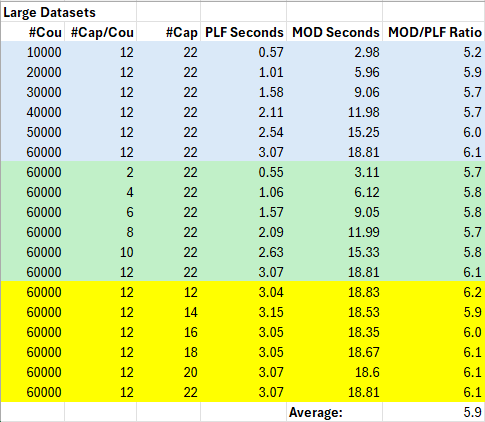
Results Table

- Straight lines provide a good match for the variation of elapsed time with #Cou for both PLF and MOD
- The coefficient of determination is consistent with these observations, with 0.999 indicating a good match for both straight lines
- PLF is about 6 times faster than MOD after the first data point, where it was about 5 times faster
Results Graph
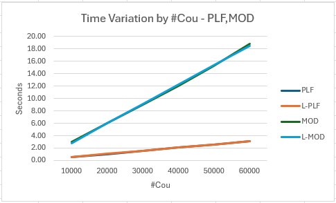
- The graph shows the close match between observed times and the fitted lines
- It also shows PLF as consistently faster than MOD
RSF
Results Table
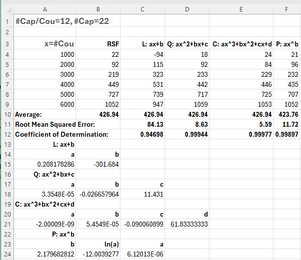
- The elapsed time for RSF seems to increase faster than quadratically with #Cou
- Polynomials of order 1, 2 and 3 and a power-law curve were fitted
- The smallest root mean squared error was for the cubic curve
- The quadratic curve was not far behind, with the power-law curve slightly worse
- The linear curve was much worse than the others
- The coefficient of determination is consistent with these observations, with 0.99977 for the cubic curve indicating a good match
Results Graph
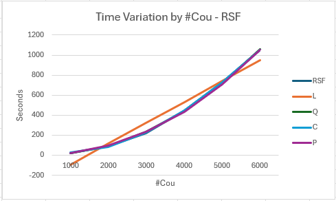
- The graph shows RSF as the observed times, with the four fitted curves
- All apart from the straight line show reasonable matches with the observed values on the graph, although the tabulated figures above allow differentiation
Time Variation by #Cap/Cou
PLF, MOD
Results Table
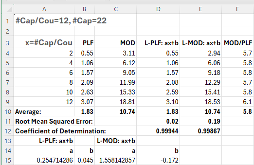
- Straight lines provide a good match for the variation of elapsed time with #Cap/Cou for both PLF and MOD
- The coefficient of determination is consistent with these observations, with 0.999 indicating a good match for both straight lines
- PLF is consistently about 6 times faster than MOD
Results Graph
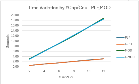
- The graph shows the close match between observed times and the fitted lines
- It also shows PLF as consistently faster than MOD
RSF
Results Table
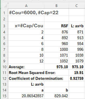
- The elapsed time for RSF seems to vary approximately linearly with #Cap/Cou
- The coefficient of determination, at 0.93, is not quite as high as some of the other straight line fits
Results Graph
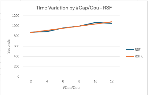
- The graph shows a moderately close match between observed times and the fitted line
Time Variation by #Cap
PLF, MOD
Results Table
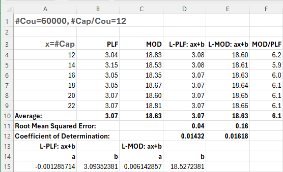
- The elapsed times are approximately constant with #Cap for both PLF and MOD
- Although the root mean squared errors at 0.04 and 0.16 for the two fitted lines, respectively, are quite small, the coefficients of determination at 0.014 and 0.016 are much lower than in earlier case
- I guess this just indicates that fitting lines adds little value in this case compared with just taking the mean values; in fact, taking the mean values might actually be better if the variations are just random noise
- PLF is again consistently about 6 times faster than MOD
Results Graph
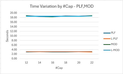
- The graph shows the observed times are close to constant, as are the fitted lines
RSF
Results Table

- The elapsed time for RSF seems to vary linearly with #Cap/Cou to a good approximation
- The coefficient of determination, at 0.9997, is very high here
Results Graph

- The graph shows a close match between observed times and the fitted line
Analysis of Results
↑ Results
↓ PLF
↓ MOD
↓ RSF
↓ Summary
PLF
Execution Plans
- Dataset parameters: #Cou = 60000, #Cap/Cou = 12, #Cap = 22
The pipelined function has two execution plans: The first is for the top-level SQL and is not very informative, because most of the work is done in the lower level SQL and PL/SQL within the function itself.
-----------------------------------------------------------------------------------------------------------------------
| Id  | Operation                           | Name                  | Starts | E-Rows | A-Rows |   A-Time   | Buffers |
-----------------------------------------------------------------------------------------------------------------------
|   0 | SELECT STATEMENT                    |                       |      1 |        |      1 |00:00:03.23 |    2592 |
|   1 |  VIEW                               | COUPON_CAPS_PLF_AGG_V |      1 |      1 |      1 |00:00:03.23 |    2592 |
|   2 |   SORT AGGREGATE                    |                       |      1 |      1 |      1 |00:00:03.23 |    2592 |
|   3 |    COLLECTION ITERATOR PICKLER FETCH| CAPS                  |      1 |   8168 |    720K|00:00:05.74 |    2592 |
-----------------------------------------------------------------------------------------------------------------------
- The A-Rows of 720K in step 3 represents all the rows returned before aggregation and equals #Cou * #Cap/Cou
- Note the estimated E-Rows of 8168 is a default used by Oracle’s SQL engine when it has no cardinality estimate, as here when a pipelined function is called
- The poor estimate does not matter in this case
This is the execution plan obtained by running the function cursor separately against the largest dataset (script: get_plf_xplan.sql):
--------------------------------------------------------------------------------------------------------------------------------
| Id  | Operation            | Name               | Starts | E-Rows | A-Rows |   A-Time   | Buffers |  OMem |  1Mem | Used-Mem |
--------------------------------------------------------------------------------------------------------------------------------
|   0 | SELECT STATEMENT     |                    |      1 |        |    720K|00:00:01.09 |    3022 |       |       |          |
|   1 |  SORT ORDER BY       |                    |      1 |  72000 |    720K|00:00:01.09 |    3022 |    40M|  2253K|   35M (0)|
|*  2 |   HASH JOIN          |                    |      1 |  72000 |    720K|00:00:00.14 |    3022 |  4656K|  2259K| 4679K (0)|
|   3 |    TABLE ACCESS FULL | COUPON_DATA        |      1 |   6000 |  60000 |00:00:00.01 |     247 |       |       |          |
|*  4 |    HASH JOIN         |                    |      1 |  72000 |    720K|00:00:00.08 |    2775 |  1744K|  1744K| 1435K (0)|
|   5 |     TABLE ACCESS FULL| CAP_DATA           |      1 |     20 |     22 |00:00:00.01 |       6 |       |       |          |
|   6 |     TABLE ACCESS FULL| COUPON_CAP_MAPPING |      1 |  72000 |    720K|00:00:00.04 |    2769 |       |       |          |
--------------------------------------------------------------------------------------------------------------------------------
Predicate Information (identified by operation id):
---------------------------------------------------
2 - access("COU"."COUPON"="CCM"."COUPON")
4 - access("CCM"."CAP_NAME"="CAP"."CAP_NAME")
- The plan here is simply two hash joins reading all data from the tables
- As the COUPON_DATA and CAP_DATA are joined in step 4 via the intersection table, COUPON_CAP_MAPPING, the overall A-Rows equals #Cou * #Cap/Cou
- Reading the 22 records in CAP_DATA takes a negligible time, which would not vary significantly across the #Cap parameter range
- This explains why PLF shows roughly constant time across #Cap
- The time might be expected to be proportional to the rows returned before aggregation, and thus be linear in #Cou and #Cap/Cou, which the actual results bear out
MOD
- Dataset parameters: #Cou = 60000, #Cap/Cou = 12, #Cap = 22
Execution Plan
----------------------------------------------------------------------------------------------------------------------------------------------------------------------
| Id  | Operation                   | Name                  | Starts | E-Rows | A-Rows |   A-Time   | Buffers | Reads  | Writes |  OMem |  1Mem | Used-Mem | Used-Tmp|
----------------------------------------------------------------------------------------------------------------------------------------------------------------------
|   0 | SELECT STATEMENT            |                       |      1 |        |      1 |00:00:18.50 |    2592 |   4995 |   4995 |       |       |          |         |
|   1 |  VIEW                       | COUPON_CAPS_MOD_AGG_V |      1 |      1 |      1 |00:00:18.50 |    2592 |   4995 |   4995 |       |       |          |         |
|   2 |   SORT AGGREGATE            |                       |      1 |      1 |      1 |00:00:18.50 |    2592 |   4995 |   4995 |       |       |          |         |
|   3 |    VIEW                     | COUPON_CAPS_MOD_V     |      1 |    716K|    720K|00:00:18.59 |    2592 |   4995 |   4995 |       |       |          |         |
|   4 |     SQL MODEL ORDERED FAST  |                       |      1 |    716K|    720K|00:00:18.42 |    2592 |   4995 |   4995 |   103M|  9043K|  101M (0)|         |
|   5 |      WINDOW SORT            |                       |      1 |    716K|    720K|00:00:04.47 |    2592 |   4995 |   4995 |    50M|  2494K|   44M (0)|         |
|   6 |       WINDOW SORT           |                       |      1 |    716K|    720K|00:00:02.64 |    2592 |   4995 |   4995 |    44M|  2348K|   39M (0)|         |
|   7 |        VIEW                 |                       |      1 |    716K|    720K|00:00:00.92 |    2592 |   4995 |   4995 |       |       |          |         |
|   8 |         WINDOW SORT         |                       |      1 |    716K|    720K|00:00:00.92 |    2592 |   4995 |   4995 |    43M|  2339K|   45M (1)|      40M|
|*  9 |          HASH JOIN          |                       |      1 |    716K|    720K|00:00:00.14 |    2589 |      0 |      0 |  1744K|  1744K| 1444K (0)|         |
|  10 |           TABLE ACCESS FULL | CAP_DATA              |      1 |     22 |     22 |00:00:00.01 |       7 |      0 |      0 |       |       |          |         |
|* 11 |           HASH JOIN         |                       |      1 |    716K|    720K|00:00:00.09 |    2582 |      0 |      0 |  4656K|  2259K| 4602K (0)|         |
|  12 |            TABLE ACCESS FULL| COUPON_DATA           |      1 |  60000 |  60000 |00:00:00.01 |     203 |      0 |      0 |       |       |          |         |
|  13 |            TABLE ACCESS FULL| COUPON_CAP_MAPPING    |      1 |    720K|    720K|00:00:00.03 |    2379 |      0 |      0 |       |       |          |         |
----------------------------------------------------------------------------------------------------------------------------------------------------------------------

Predicate Information (identified by operation id):
---------------------------------------------------

   9 - access("CCM"."CAP_NAME"="CAP"."CAP_NAME")
  11 - access("COU"."COUPON"="CCM"."COUPON")
- The inner query on the three tables is executed using a similar pair of hash joins to PLF, except the join order differs, with CAP_DATA and COUPON_DATA swapped
- We’d expect similar linear variation across #Cou and #Cap/Cou as in PLF, and constancy across #Cap
- Although the variations are of the same kind as in PLF, MOD typically takes 6 times as long
- Most of the work seems to be done in step 6, ‘SQL MODEL ORDERED FAST’, confirming the reputation of the MODEL clause for adding a lot of overhead in queries
RSF
- Dataset parameters: #Cou = 6000, #Cap/Cou = 12, #Cap = 22
Execution Plan
----------------------------------------------------------------------------------------------------------------------------------------------------------
| Id  | Operation                                   | Name                  | Starts | E-Rows | A-Rows |   A-Time   | Buffers |  OMem |  1Mem | Used-Mem |
----------------------------------------------------------------------------------------------------------------------------------------------------------
|   0 | SELECT STATEMENT                            |                       |      1 |        |      1 |00:18:19.51 |     363M|       |       |          |
|   1 |  VIEW                                       | COUPON_CAPS_RSF_AGG_V |      1 |      1 |      1 |00:18:19.51 |     363M|       |       |          |
|   2 |   SORT AGGREGATE                            |                       |      1 |      1 |      1 |00:18:19.51 |     363M|       |       |          |
|*  3 |    VIEW                                     |                       |      1 |     61T|  72000 |00:48:28.06 |     363M|       |       |          |
|   4 |     UNION ALL (RECURSIVE WITH) BREADTH FIRST|                       |      1 |        |    132K|00:21:26.35 |     363M|  2048 |  2048 |  299K (0)|
|   5 |      TABLE ACCESS FULL                      | CAP_DATA              |      1 |     22 |     22 |00:00:00.01 |       7 |       |       |          |
|   6 |      WINDOW SORT                            |                       |   6001 |     61T|    132K|00:03:57.73 |    1488K|  4096 |  4096 | 4096  (0)|
|   7 |       MERGE JOIN OUTER                      |                       |   6001 |     61T|    132K|00:03:57.73 |    1488K|       |       |          |
|   8 |        SORT JOIN                            |                       |   6001 |     61T|    132K|00:00:12.97 |     275 |  4096 |  4096 | 4096  (0)|
|*  9 |         HASH JOIN                           |                       |   6001 |     61T|    132K|00:00:12.62 |     275 |  1506K|  1506K| 1725K (0)|
|  10 |          BUFFER SORT (REUSE)                |                       |   6001 |        |     36M|00:00:03.54 |     274 |   337K|   337K|  299K (0)|
|  11 |           VIEW                              |                       |      1 |   6000 |   6000 |00:00:00.02 |     274 |       |       |          |
|  12 |            WINDOW SORT                      |                       |      1 |   6000 |   6000 |00:00:00.02 |     274 |   232K|   232K|  206K (0)|
|* 13 |             HASH JOIN SEMI                  |                       |      1 |   6000 |   6000 |00:00:00.02 |     274 |  1695K|  1695K| 1620K (0)|
|  14 |              TABLE ACCESS FULL              | COUPON_DATA           |      1 |   6000 |   6000 |00:00:00.01 |      23 |       |       |          |
|  15 |              INDEX FAST FULL SCAN           | CCM_PK                |      1 |  72000 |  71980 |00:00:00.01 |     251 |       |       |          |
|* 16 |          HASH JOIN                          |                       |   6001 |   1026G|    132K|00:00:01.08 |       1 |  1506K|  1506K| 1628K (0)|
|  17 |           BUFFER SORT (REUSE)               |                       |   6001 |        |    132K|00:00:00.05 |       1 | 73728 | 73728 |          |
|  18 |            INDEX FULL SCAN                  | CAP_PK                |      1 |     22 |     22 |00:00:00.01 |       1 |       |       |          |
|  19 |           RECURSIVE WITH PUMP               |                       |   6001 |        |    132K|00:00:00.05 |       0 |       |       |          |
|* 20 |        SORT JOIN                            |                       |    132K|  72000 |  72000 |00:03:43.84 |    1488K|  3313K|   798K| 2944K (0)|
|  21 |         TABLE ACCESS FULL                   | COUPON_CAP_MAPPING    |   6000 |  72000 |    432M|00:01:20.09 |    1488K|       |       |          |
----------------------------------------------------------------------------------------------------------------------------------------------------------

Predicate Information (identified by operation id):
---------------------------------------------------

   3 - filter(("COUPON" IS NOT NULL AND "CAP_SEQUENCE" IS NOT NULL))
   9 - access("COU"."COU_IND"="RSF"."COU_IND"+1)
  13 - access("CCM"."COUPON"="COU"."COUPON")
  16 - access("CAP"."CAP_NAME"="RSF"."CAP_NAME")
  20 - access("CCM"."COUPON"="COU"."COUPON" AND "CCM"."CAP_NAME"="RSF"."CAP_NAME")
       filter(("CCM"."CAP_NAME"="RSF"."CAP_NAME" AND "CCM"."COUPON"="COU"."COUPON"))
- There is an iteration within the recursion for each coupon, and this would suggest an initial factor of #Cou in the work done
- Within each iteration COUPON_DATA has ‘TABLE ACCESS FULL’ at step 14, which would suggest a second factor of #Cou
- In addition, step 15 has ‘INDEX FAST FULL SCAN’ on CCM_PK, whose size depends on #Cou
- These factors would seem to partially explain the greater than quadratic variation of time with #Cou for RSF
- The ‘TABLE ACCESS FULL’ on COUPON_CAP_MAPPING in step 21, without other instances, no doubt accounts for the linear variation with #Cap/Cou
- Unlike with PLF and MOD, there is also a linear variation with #Cap
- This can be explained by the need to process a row for every cap at each iteration, in order to keep track of the cap_left values
Summary
- The results show that the solution by recursive subquery factoring is much slower than by the MODEL clause, which is itself much slower than by the pipelined function.
- Both PLF and MOD show linear variation in two parameters, and no variation in the third
- RSF shows linear variation in two parameters, and worse than quadratic in the other
Unit Testing
↑ Contents
↓ Unit Testing Process
↓ Unit Test Results
The queries are tested through views using The Math Function Unit Testing Design Pattern. A ‘pure’ wrapper function is constructed that takes input parameters and returns a value, and is tested within a loop over scenario records read from a JSON file.
Unit Testing Process
↑ Unit Testing
↓ Step 1: Create Input Scenarios File
↓ Step 2: Create Results Object
↓ Step 3: Format Results
This section details the three steps involved in following The Math Function Unit Testing Design Pattern.
Step 1: Create Input Scenarios File
↑ Unit Testing Process
↓ Unit Test Wrapper Functions
↓ Scenario Category ANalysis (SCAN)
↓ Creating the Input Scenarios File
Unit Test Wrapper Functions
↑ Step 1: Create Input Scenarios File
The three queries are tested by means of views, of which only three of the projected columns need to be used as outputs in unit testing:
- coupon
- cap
- usage
The inputs are the records in the three tables. We need a separate wrapper function for each of the views tested, although they will share most of the code. There is a view for each of the three queries, and we have added a fourth view based on an initial version of the recursive query that appeared to work at first, but in some scenarios gave incorrect results. This demonstrates regression testing. The views are:
- COUPON_CAPS_PLF_V: Pipelined function
- COUPON_CAPS_MOD_V: MODEL clause
- COUPON_CAPS_RSF_V: Recursive subquery factors
- COUPON_CAPS_RSF_BUG_V: Recursive subquery factors, with bug
The diagram below shows the structure of the input and output of the wrapper functions.

From the input and output groups depicted we can construct CSV files with flattened group/field structures, and default values added, as follows:
coupon_caps_inp.csv
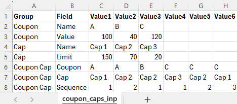
The value fields shown correspond to a prototype scenario with records per input group:
- Coupon: 3
- Cap: 3
- Coupon Cap: 6
coupon_caps_out.csv
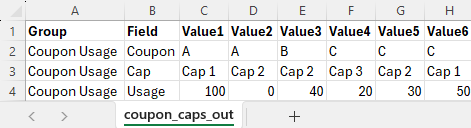
The value fields shown correspond to a prototype scenario with records per output group:
- Coupon Usage: 6
A PowerShell utility uses these CSV files, together with one for scenarios, discussed next, to generate a template for the JSON unit testing input file. The utility creates a prototype scenario with a record in each group for each populated value column.
Scenario Category ANalysis (SCAN)
↑ Step 1: Create Input Scenarios File
↓ Generic Category Sets
↓ Categories and Scenarios
The art of unit testing lies in choosing a set of scenarios that will produce a high degree of confidence in the functioning of the unit under test across the often very large range of possible inputs.
A useful approach to this can be to think in terms of categories of inputs, where we reduce large ranges to representative categories. I explore this approach further in this article:
Generic Category Sets
↑ Scenario Category ANalysis (SCAN)
As explained in the article mentioned above, it can be very useful to think in terms of generic category sets that apply in many situations. Multiplicity is relevant here (as it often is):
Multiplicity
There are two entities where the generic category set of multiplicity applies, and we should check each of the One / Multiple instance categories.
| Code | Description |
|---|---|
| 1 | One value |
| Multiple | Multiple values |
Apply to:
- Coupon Usage
- Cap Usage
There is also a second kind of multiplicity for combinations of entities (X, Y), applying here to (Coupon, Cap):
| Code | Description |
|---|---|
| 1 - 1 | One X, One Y |
| 1 - Multiple | One X, Multiple Y |
| Multiple - 1 | Multiple X, One Y |
| Multiple - Multiple | Multiple X, Multiple Y |
Categories and Scenarios
↑ Scenario Category ANalysis (SCAN)
After analysis of the possible scenarios in terms of categories and category sets, we can depict them on a Category Structure diagram:
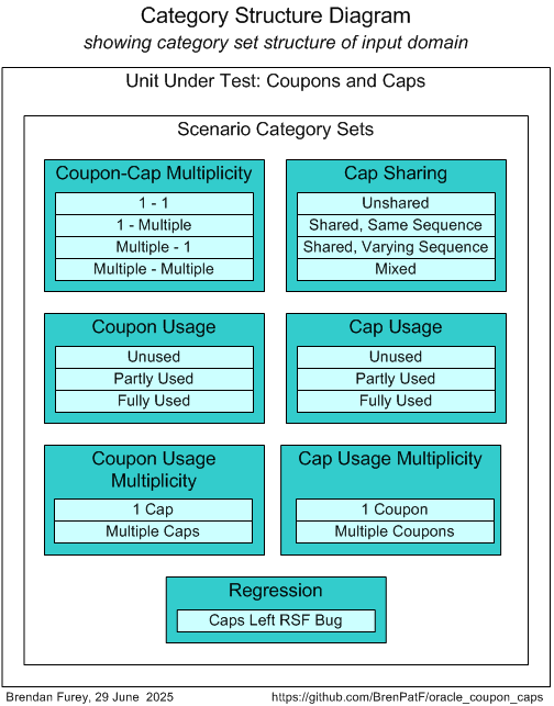
Note that the last category set, Regression, is used for regression testing, with a single category corresponding to a bug found in an initial version of the recursive query.
We can tabulate the results of the category analysis, and assign a scenario against each category set/category with a unique description:
| # | Category Set | Category | Scenario |
|---|---|---|---|
| 1 | Coupon-Cap Multiplicity | 1 - 1 | One coupon, one cap |
| 2 | Coupon-Cap Multiplicity | 1 - Multiple | One coupon, multiple caps |
| 3 | Coupon-Cap Multiplicity | Multiple - 1 | Multiple coupons, one cap |
| 4 | Coupon-Cap Multiplicity | Multiple - Multiple | Multiple coupons, multiple caps |
| 5 | Cap Sharing | Unshared | Caps unshared |
| 6 | Cap Sharing | Shared, Same Sequence | Caps shared using same sequences |
| 7 | Cap Sharing | Shared, Varying Sequence | Caps shared using varying sequences |
| 8 | Cap Sharing | Mixed | Some caps unshared, and some shared |
| 9 | Coupon Usage | Unused | Coupon unused |
| 10 | Coupon Usage | Partly Used | Coupon partly used |
| 11 | Coupon Usage | Fully Used | Coupon fully used |
| 12 | Cap Usage | Unused | Cap unused |
| 13 | Cap Usage | Partly Used | Cap partly used |
| 14 | Cap Usage | Fully Used | Cap fully used |
| 15 | Coupon Usage Multiplicity | 1 Cap | One cap used per coupon |
| 16 | Coupon Usage Multiplicity | Multiple Caps | Multiple caps used per coupon |
| 17 | Cap Usage Multiplicity | 1 Coupon | One coupon used per cap |
| 18 | Cap Usage Multiplicity | Multiple Coupons | Multiple coupons used per cap |
| 19 | Regression | Caps Left RSF Bug | Caps left RSF bug |
From the scenarios identified we can construct the following CSV file, taking the category set and scenario columns, and adding an initial value for the active flag:
coupon_caps_sce.csv

Creating the Input Scenarios File
↑ Step 1: Create Input Scenarios File
The powershell API to generate a template JSON file can be run with the following powershell in the folder of the CSV files:
Format-JSON-Coupon_Caps.ps1
Import-Module TrapitUtils
Write-UT_Template 'coupon_caps' '|'
This creates the template JSON file, coupon_caps_temp.json, which contains an element for each of the scenarios, with the appropriate category set and active flag, and a prototype set of input and output records.
In the prototype record sets, each group has zero or more records with field values taken from the group CSV files, with a record for each value column present where at least one value is not null for the group. The template scenario records may be manually updated (and added or subtracted) to reflect input and expected output values for the actual scenario being tested.
Load JSON File into Database
A record is added into the table TT_UNITS by a call to the Trapit.Add_Ttu API for each view, as shown. The input JSON file must first be placed in the operating system folder pointed to by the INPUT_DIR directory, and is loaded into a JSON column in the table. The name of the unit test package (‘TT_COUPON_CAPS’), the functions (‘Coupon_Caps_MOD’ etc.), the unit test group (‘coupon_caps’), and the titles are also passed.
DECLARE
  l_api_lis L1_Chr_Arr := L1_Chr_Arr(
      'Coupon_Caps_MOD',
      'Coupon_Caps_RSF',
      'Coupon_Caps_RSF_Bug',
      'Coupon_Caps_PLF'
  );
  PROCEDURE Add_API (p_purely_wrap_api_function_nm  VARCHAR2) IS
  BEGIN
    Trapit.Add_Ttu(
            p_unit_test_package_nm         => 'TT_COUPON_CAPS',
            p_purely_wrap_api_function_nm  => p_purely_wrap_api_function_nm,
            p_group_nm                     => 'coupon_caps',
            p_active_yn                    => 'Y',
            p_input_file                   => 'tt_coupon_caps.purely_wrap_coupon_caps_inp.json',
            p_title                        => 'Coupon Caps - ' || CASE p_purely_wrap_api_function_nm
                                                                       WHEN 'Coupon_Caps_MOD'     THEN 'Model Clause'
                                                                       WHEN 'Coupon_Caps_RSF'     THEN 'Recursive Query'
                                                                       WHEN 'Coupon_Caps_RSF_Bug' THEN 'Recursive Query, with bug'
                                                                       ELSE                            'Pipelined Function' END
    );
  END Add_API;
BEGIN
  FOR i IN 1..l_api_lis.COUNT LOOP
    Add_API(l_api_lis(i));
  END LOOP;
END;
/
Step 2: Create Results Object
Step 2 requires the writing of a wrapper function that is called by a library packaged procedure that runs all tests for a group name passed in as a parameter. In this case we have a package containing a wrapper function for each view, with each one calling a private function passing in the view name along with the standard input parameter. The extract shows the code for the function Coupon_Caps_MOD, with the private function called. The latter function calls three private procedures to insert the test data based on the p_inp_3lis parameter.
TT_Coupon_Caps (extract from package body)
FUNCTION purely_Wrap_Cou_Caps(
              p_view_name                    VARCHAR2,
              p_inp_3lis                     L3_chr_arr)
              RETURN                         L2_chr_arr IS
  l_act_2lis        L2_chr_arr := L2_chr_arr();
  l_result_lis      L1_chr_arr;
BEGIN
  DELETE coupon_data;
  DELETE cap_data;
  DELETE coupon_cap_mapping;
  add_Cous     (p_cou_2lis     => p_inp_3lis(1));
  add_Caps     (p_cap_2lis     => p_inp_3lis(2));
  add_Cou_Caps (p_cou_cap_2lis => p_inp_3lis(3));
  l_act_2lis.EXTEND;
  l_act_2lis(1) := Utils.View_To_List(
                                p_view_name     => p_view_name,
                                p_sel_value_lis => L1_chr_arr('coupon', 'cap_name', 'usage'),
                                p_where         => '1=1',
                                p_order_by      => 'coupon, cap_sequence');
  ROLLBACK;
  RETURN l_act_2lis;
END purely_Wrap_Cou_Caps;

FUNCTION Coupon_Caps_MOD(
              p_inp_3lis                     L3_chr_arr)
              RETURN                         L2_chr_arr IS
BEGIN
    RETURN purely_Wrap_Cou_Caps(
              p_view_name   => 'coupon_caps_mod_v',
              p_inp_3lis    => p_inp_3lis);
END Coupon_Caps_MOD;
Step 3: Format Results
Step 3 involves formatting the results contained in the JSON output file from step 2, via the JavaScript formatter, and this step can be combined with step 2 for convenience.
Test-FormatDBis the function from the TrapitUtils PowerShell package that calls the main test driver function, then passes the output JSON file name to the JavaScript formatter and outputs a summary of the results.
Test-Format-Coupon_Caps.ps1
Import-Module ..\powershell_utils\TrapitUtils\TrapitUtils
Test-FormatDB 'app/app' 'orclpdb' 'coupon_caps' $PSScriptRoot `
'BEGIN
    Utils.g_w_is_active := FALSE;
END;
/
'
This script calls the TrapitUtils library function Test-FormatDB, passing in for the preSQL parameter a SQL string to turn off logging to spool file.
Unit Test Results
↑ Unit Testing
↓ Unit Test Report: Coupon Caps - Recursive Query, with bug
↓ Results for Scenario 19: Caps left RSF bug [Category Set: Regression]
The unit test script creates a results subfolder for each unit in the ‘coupon_caps’ group, with results in text and HTML formats, in the script folder, and outputs the following summary:
File:          tt_coupon_caps.coupon_caps_mod_out.json
Title:         Coupon Caps - Model Clause
Inp Groups:    3
Out Groups:    2
Tests:         19
Fails:         0
Folder:        coupon-caps---model-clause

File:          tt_coupon_caps.coupon_caps_rsf_out.json
Title:         Coupon Caps - Recursive Query
Inp Groups:    3
Out Groups:    2
Tests:         19
Fails:         0
Folder:        coupon-caps---recursive-query

File:          tt_coupon_caps.coupon_caps_rsf_bug_out.json
Title:         Coupon Caps - Recursive Query, with bug
Inp Groups:    3
Out Groups:    2
Tests:         19
Fails:         1
Folder:        coupon-caps---recursive-query,-with-bug

File:          tt_coupon_caps.coupon_caps_plf_out.json
Title:         Coupon Caps - Pipelined Function
Inp Groups:    3
Out Groups:    2
Tests:         19
Fails:         0
Folder:        coupon-caps---pipelined-function
You can review the full HTML formatted unit test results here for the four views tested:
- Unit Test Report: Coupon Caps - Model Clause
- Unit Test Report: Coupon Caps - Recursive Query
- Unit Test Report: Coupon Caps - Recursive Query, with bug
- Unit Test Report: Coupon Caps - Pipelined Function
Next we show the scenario-level summary of results for the view with a bug.
Unit Test Report: Coupon Caps - Recursive Query, with bug
Here is the results summary in HTML format for the view with a bug:

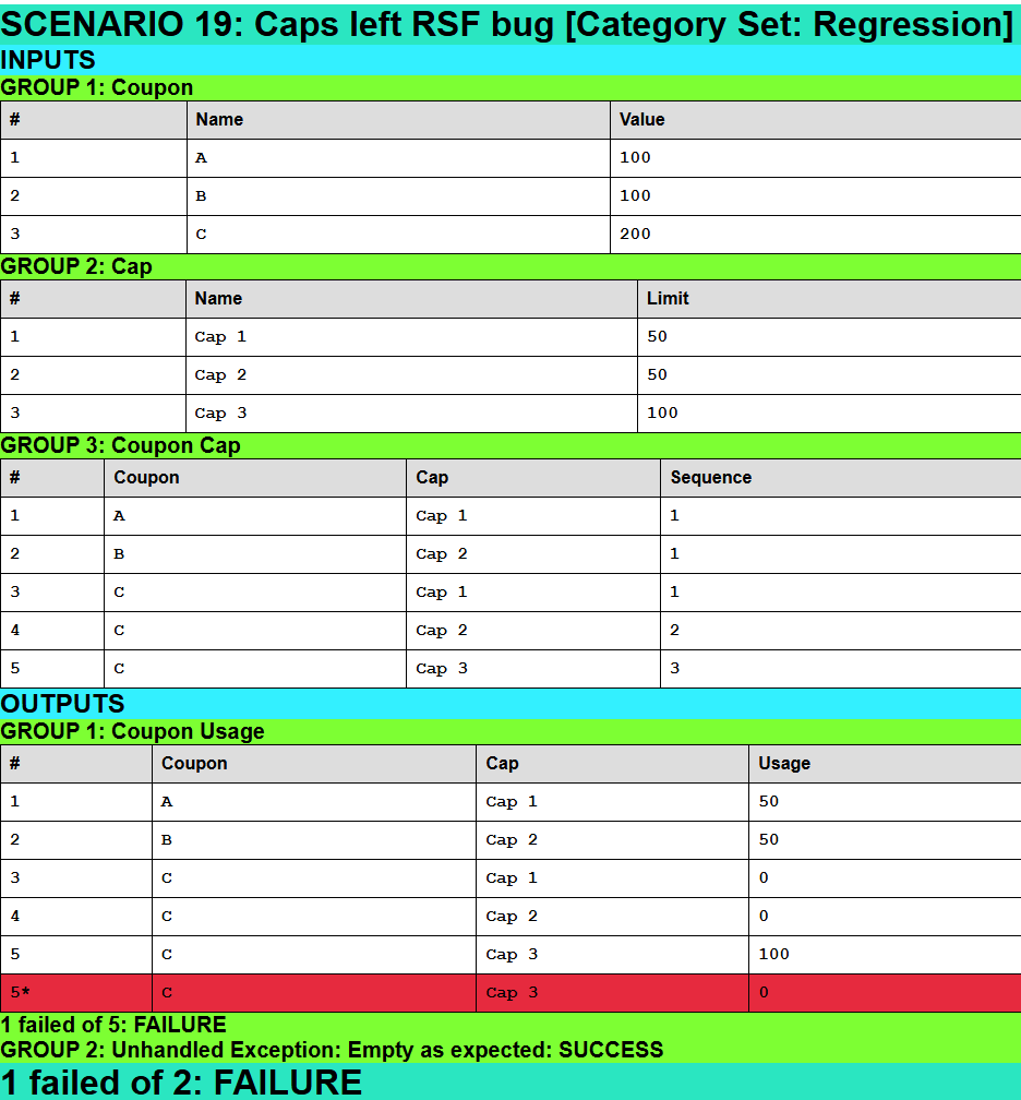
Results for Scenario 19: Caps left RSF bug [Category Set: Regression]
Here is the results page for scenario 19 in HTML format for the view with a bug:
Conclusion
In this article we demonstrated how to solve the Coupons and Caps Allocation Problem by three distinct SQL and PL/SQL techniques:
- Pipelined functions
- The MODEL clause
- Recursive subquery factoring
We analysed the performance characteristics of each method using Dimensional Performance Benchmarking of SQL, supported by Excel graphs and statistical functions for curve-fitting.
As with earlier articles - Shortest Path Analysis of Large Networks by SQL and PL/SQL and OPICO 6: Mixed SQL and PL/SQL Methods for Item/Category Optimization - we showed how combining SQL for set-based operations with PL/SQL for fine-grained control can yield better performance in solving algorithmic problems.
All three methods were unit tested using The Math Function Unit Testing Design Pattern. We also included a variant of one of the methods with a bug to demonstrate regression testing.
We emphasised along the way the importance of the function as an abstract concept, applying it in multiple domains.
Automation
Each of the following areas are fully automated (see the GitHub project for the code, Coupons, Caps and Functions in Oracle):
- Installation of code
- Running of the queries across all datasets, capturing execution times and execution plans
- Unit testing
See Also
- Solving a logical problem using analytical functions
- Coupons, Caps and Functions in Oracle
- The Math Function Unit Testing Design Pattern
- Oracle PL/SQL Code Timing Module
- Unit Testing, Scenarios and Categories: The SCAN Method
- Shortest Path Analysis of Large Networks by SQL and PL/SQL
- OPICO 6: Mixed SQL and PL/SQL Methods for Item/Category Optimization
- Least squares
- Coefficient of determination
- Kraftwerk